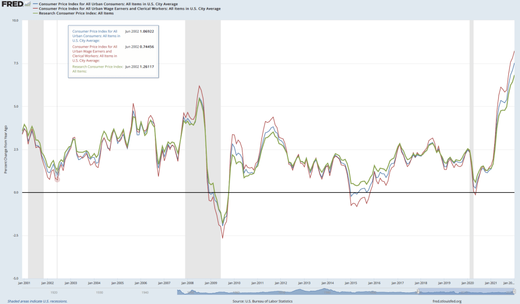
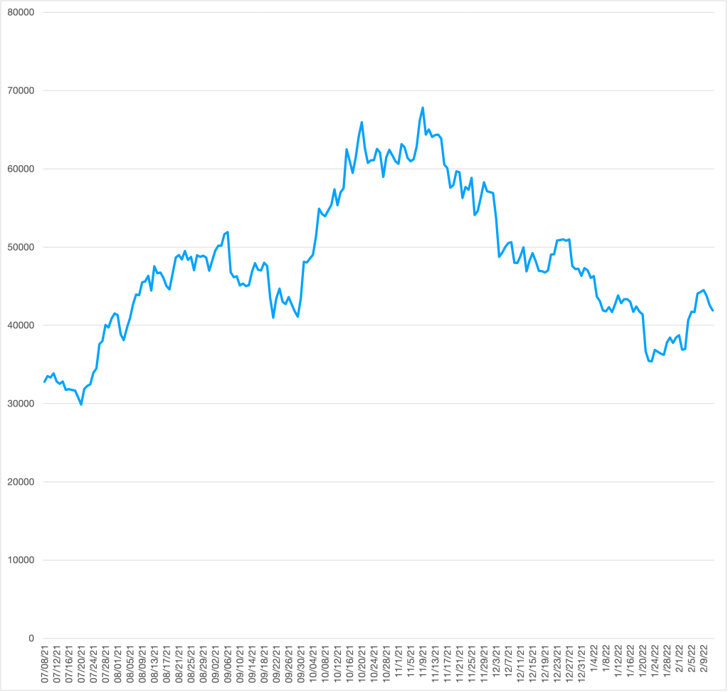
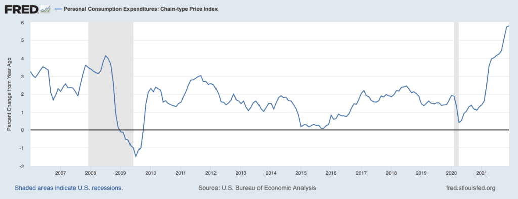
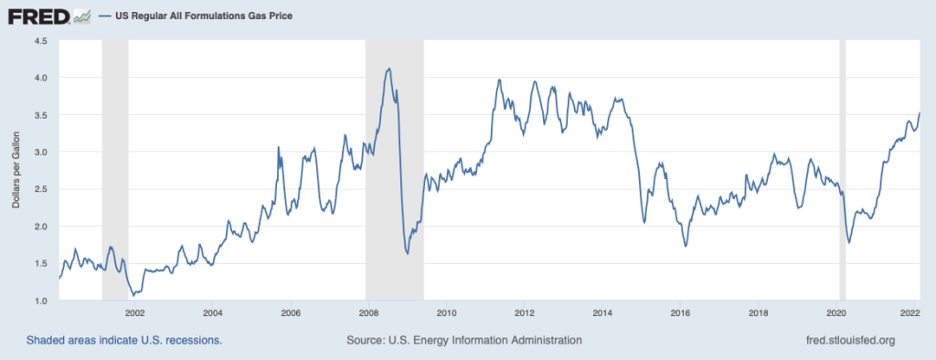
The National Debt Just Hit $30 Trillion. Who Owns It?

On February 1, 2022, a headline in the Wall Street Journal noted that: “U.S. National Debt Exceeds $30 Trillion for the First Time.” The national debt—or, more formally, the federal government debt—is the value of all U.S. Treasury securities outstanding. Treasury securities include Treasury bills, which mature in one year or less; Treasury notes, which mature between 2 years and 10 years; Treasury bonds, which mature in 30 years; U.S. savings bonds purchased by individual investors; and Treasury Inflation-Protected Securities (TIPS), which, unlike other Treasury securities, have their principal amounts adjusted every six months to reflect changes in the consumer price index (CPI).  

With a value of $30 trillion, the federal government debt in early February is about 120 percent of GDP, a record that exceeds the ratio of government debt to GDP during World War II. In 2007, at the beginning of the Great Recession of 2007–2009, the ratio of government debt to GDP was only 35 percent. (We discuss the federal government debt in Macroeconomics, Chapter 16, Section 16.6 and in Economics, Chapter 26, Section 26.6.)

There are many important economic issues involved with the federal government debt, but in this blog post we’ll focus just on the question of who owns the debt.

The pie chart below shows the shares of the debt held by different groups. The largest slice shown is for “intragovernmental holdings,” which represent ownership of Treasury securities by government trust funds, notably the Social Security trust funds. The Social Security system makes payments to retired or disabled workers. The system operates on a pay-as-you-go basis, which means that the payroll taxes collected from today’s workers are used to make payments to retired workers. Because of slowing population growth, Congress authorized an increase in payroll taxes above the level necessary to make current payments. The Social Security system has invested the surplus in special Treasury securities that the Treasury redeems when the funds are necessary to make payments to retired workers. (In the Apply the Concept “Is Spending on Social Security and Medicare a Fiscal Time Bomb?” in Macroeconomics, Chapter 16, Section 16.1, we discuss the long-term funding problems of the Social Security and Medicare systems.)

Some economists argue that the value of these Treasury securities should not be counted as part of the federal government debt because the securities are not marketable in the way that Treasury bills, notes, and bonds are and because the securities represent a flow of funds from one federal agency to another federal agency. If we exclude the value of these securities, the national debt on February 1, 2022 was $23.5 trillion rather than $30.0 trillion. 

The Federal Reserve System holds about 19 percent of federal government debt. The Fed buys and sells Treasury securities as part of its normal conduct of monetary policy. In addition, the Fed accumulated large holdings of Treasury securities as part of its quantitative easing operations during and following the 2007–2009 financial crisis and from 2020 to 2022 during the worst of the Covid-19 pandemic. (We discuss quantitative easing in Macroeconomics, Chapter 15, Section 15.3.)

About 27 percent of the debt is held by foreign central banks, foreign commercial banks, and foreign investors. The largest amount of Treasury debt is held by Japan, followed by China and the United Kingdom. All other countries combined hold about 16 percent of the debt.

U.S. commercial banks hold more than 15 percent of the debt. Banks hold Treasury securities partly because since the 2007–2009 financial crisis most interest rates, including those on loans and on corporate and municipal bonds, have been very low compared with historic averages. The interest rates on these assets are in some cases too low to compensate banks for the risk of owning the assets rather than default-risk free Treasury securities. In addition, large banks are required to meet a liquidity coverage ratio, which means that they have to hold sufficient liquid assets—those that can be easily converted into cash—to meet their need for funds in a financial crisis. Many banks meet their liquidity requirements, in part, by owning Treasury securities. 

The remaining Treasury securities—about 16.5 percent of the total federal government debt—are held by the U.S. nonbank public. The nonbank public includes financial firms—such as investment banks, insurance companies, and mutual funds—as well as individual investors.

Sources: Amara Omeokwe, “U.S. National Debt Exceeds $30 Trillion for First Time,” Wall Street Journal, February 1, 2022; “Debt to the Penny,” fiscaldata.treasury.gov; “Major Foreign Holders of Treasury Securities,” ticdata.treasury.gov; and Federal Reserve Bank of St. Louis.

The Surprisingly Strong Employment Report for January 2022

Leisure and hospitality was one of the industries showing surprisingly strong job growth during January 2022. Photo from the New York Times.

The Bureau of Labor Statistics’ monthly report on the “Employment Situation” is generally considered the best source of information on the current state of the labor market. As we discuss in Macroeconomics, Chapter 9, Section 9.1 (and in Economics, Chapter 19, Section 19.1), economists, policymakers, and investors generally focus more on the establishment survey data on total payroll employment than on the household survey data on the unemployment rate. The initial data on employment from the establishment survey are subject to substantial revisions over time (we discuss this point further below). But the establishment survey has the advantage of being determined by data taken from actual payrolls rather than by unverified answers to survey questions, as is the case with the household survey data. 

The establishment survey data for January 2022 (released on February 4, 2022) showed a surprisingly large increase in employment of 467,000. The consensus forecast had been for a significantly smaller increase of 150,000, with many economists expecting that the data would show a decrease in employment. The establishment survey is collected for pay periods that include the 12th of the month. In January 2022, in many places in the United States that pay period coincided with the height of the wave of infections from the Omicron variant of Covid-19. And, in fact, according to the household survey, the number of people out of work because of illness was 3.6 million in January—the most during the Covid-19 pandemic. So it seemed likely that payroll employment would have declined in January. But despite the difficulties caused by the pandemic, payroll employment increased substantially, likely reflecting firms’ continuing high demand for workers—a demand reflected in the very high level of job openings.

The employment report includes the BLS’s annual data revisions, which are based on a comprehensive payroll count for a particular month in the previous year—in this case, March 2021. The revisions also incorporate changes to the BLS’s seasonal adjustment factors. Each month, the BLS adjusts the raw payroll employment data to reflect seasonal fluctuations such as occur during and after the end-of-year holiday period. For instance, the change from December 2020 to January 2021 in the raw employment data was −2,824,000, whereas the adjusted change was 467,000 (as noted earlier). Obviously this difference is very large and is attributable to the BLS’s seasonal adjustments removing the employment surge in December attributable to seasonal hiring by retail stores, delivery firms, and other businesses strongly affected by the holidays.

The changes to the seasonal adjustment factors made the revisions to the 2021 payroll employment numbers unusually large. For instance, the BLS initially reported that employment increased from June 2021 to July 2021 by 1,091,000, whereas the revision reduced the increase to 689,000. Table A below is reproduced from the BLS report; the figure below the table shows the changes in employment from the previous month as originally published and as revised in the January report. Overall, the BLS revisions now show that employment increased by 217,000 more from 2020 to 2021 than initially estimated. The BLS expressed the opinion that: “Going forward, the updated models should produce more reliable estimates of seasonal movements. [Because there are now] more monthly observations related to the historically large job losses and gains seen in the pandemic-driven recession and recovery, the models can better distinguish normal seasonal movements from underlying trends.”

Source: The BLS “Employment Situation” report can be found here.

Price Leadership in the Beer Market

InBev’s St. Louis production line for Stell Artois beer. Photo from the Wall Street Journal

Firms in an oligopoly can increase their profits by agreeing with other firms in the industry on what prices to charge. Explicit price fixing violates the antitrust laws and can subject the firms involved to fines of up to $100 million and executives at the firms to fines of up to $1 million and prison terms of up to 10 years. Despite these penalties, the rewards to avoiding price competition are often so great that firms look for ways to implicitly collude—that is, to arrange ways to coordinate their prices without violating the law by explicitly agreeing on the prices to charge. (We discuss the antitrust laws in Microeconomics and Economics, Chapter 15, Section 15.6.) 

One way for firms to implicitly collude is through price leadership. With price leadership, one firm in the industry takes the lead in announcing a price change that other firms in the industry then match. (We briefly discuss price leadership in Microeconomics and Economics, Chapter 14, Section 14.2.)

In their classic industrial organization textbook, F.M. Scherer of Harvard’s Kennedy School and David Ross of Bryn Mawr College summarize the legal status of price leadership, given court opinions from antitrust cases: “[P]rice leadership is not apt to be found contrary to the antitrust laws unless the leader attempts to coerce other producers into following its lead, or unless there is evidence of an agreement among members of the industry to use the leadership device as the basis of a price-fixing scheme.” As the Federal Trade Commission notes on its website: “A uniform, simultaneous price change could be the result of price fixing, but it could also be the result of independent business responses to the same market conditions.”

Scherer and Ross describe price leadership in a number of oligopolistic industries during the twentieth century, including cigarettes, steel, automobiles, breakfast cereals, turbogenerators, and gasoline.

Recently, Nathan Miller of Georgetown University, Gloria Sheu of the Federal Reserve, and Matthew Weinberg of Ohio State University published an article in the American Economic Review analyzing price leadership in the beer industry. They focus on the period from 2001 to 2011, although they believe that conditions in the beer industry are similar today. From 2001 to 2007, three large U.S.-based firms—Anheuser-Busch, SABMiller, and Molson Coors—accounted for about two-thirds of beer sales in the United States. Two importers—Heineken and Grupo Modelo—accounted for about 14 percent of sales.  In 2008, SABMiller and Molson Coors combined to form MillerCoors and InBev—which had a small market share—bought Anheuser Busch. In 2011, MillerCoors and InBev together accounted for 63 percent of beer sales.

ABI has acted as the price leader, announcing prices in the late summer that MillerCoors typically matches. ABI’s Bud Light had the largest market share among beers in the United States in 2011, well ahead of Coors Light, which had the second largest share. They find that industry profits were 17 percent above the competitive level in 2007—just before the Miller-Coors merger—and 22 percent above the competitive level in 2010—after the merger. The U.S. Department of Justice (DOJ) had decided not to contest the Miller-Coors merger because “cost savings in distribution likely would offset any loss of competition.” As it turned out, the cost savings occurred but their value was smaller than the losses in consumer surplus resulting from reduced competition.

The authors estimate that, compared with the competitive outcome, the reduction in consumer surplus in the beer market due to price leadership equaled 154 of the increase in producer surplus before the Miller-Coors merger and 170 percent after it. Figure 15.5 from Chapter 15 of Microeconomics (reproduced below) illustrates why the loss of consumer surplus is larger than the increase in producer surplus: The increase in price and decline in quantity compared with the competitive level results in a deadweight loss that reduces the total economic surplus in the market. (Note that the figure is comparing the situation when a market is monopoly with the situation when the market is perfectly competitive. For simplicity, we are assuming that price leadership in an oligopolistic industry, such as beer, results in the monopoly outcome. But note that whenever collusive behavior, like price leadership, occurs in an industry, we would expect an increase in deadweight loss that will make the gains to firms larger than the losses to consumers.)

Sources: Federal Trade Commission, “Price Fixing,” ftc.gov; U.S. Department of Justice, Antitrust Division, “Price Fixing, Bid Rigging, and Market Allocation Schemes: What They Are and What to Look for,” justice.gov; Nathan H. Miller, Gloria Sheu, and Matthew C. Weinberg, “Oligopolistic Price Leadership and Mergers: The United States Beer Industry,” American Economic Review, Vol. 111, No. 10, pp. 3123-3159; and F.M Scherer and David Ross, Industrial Market Structure and Economic Performance, Third edition, Boston: Houghton Mifflin, 1990.

AIT or FAIT: How Will the Fed’s New Monetary Policy Strategy Deal with High Inflation Rates?

Congress has given the Fed a mandate to achieve the goal of price stability. Until 2012, the Fed had never stated explicitly how they would measure whether they had achieved this goal. One interpretation of price stability is that the price level remains constant. But a constant price level would be very difficult to achieve in practice and the Fed has not attempted to do so. In 2012, the Fed, under then Chair Ben Bernanke, announced that it was targeting an inflation rate of 2 percent, which it believed was low enough to be consistent with price stability: “When households and businesses can reasonably expect inflation to remain low and stable, they are able to make sound decisions regarding saving, borrowing, and investment, which contributes to a well-functioning economy.” (We discuss inflation targeting in Macroeconomics, Chapter 15, Section 15.5 and Economics, Chapter 25, Section 25.5.)

In August 2020, the Fed announced a new monetary policy strategy that modified how it interpreted its inflation target: “[T]he Committee seeks to achieve inflation that averages 2 percent over time, and therefore judges that, following periods when inflation has been running persistently below 2 percent, appropriate monetary policy will likely aim to achieve inflation moderately above 2 percent for some time.” The Fed’s new approach is sometimes referred to as average inflation targeting (AIT) because the Fed attempts to achieve its 2 percent target on average over a period of time, although the Fed has not explicitly stated how long the period of time may be. In other words, the Fed hasn’t indicated the time horizon during which it intends inflation to average 2 percent. 

The Fed uses changes in the personal consumption expenditure (PCE) price index to measure inflation, rather than using changes in the consumer price index (CPI). The Fed prefers the PCE to the CPI because the PCE is a broader measure of the price level in that it includes the prices of more consumer goods and services than does the CPI. The following figure shows inflation for the period since 2006 measured by percentage changes in the PCE from the corresponding month in the previous year. (Members of the Fed’s Federal Open Market Committee generally consider changes in the core PCE—which excludes the prices of food and energy—to be the best measure of the underlying rate of inflation. But because the Fed’s inflation target is stated in terms of the PCE rather than the core PCE, we are looking here only at the PCE.) The figure shows that for most of the period from 2012 to early 2021, inflation was less than the Fed’s target of 2 percent.

The figure also shows that since March 2021, inflation has been running above 2 percent and has steadily increased, reaching a rate of 5.8 percent in December 2021. Note that a strict interpretation of AIT would mean that the Fed would have to balance these inflation rates far above 2 percent with future inflation rates well below 2 percent. As Ricardo Reis, an economist at the London School of Economics, noted recently: “If the [Fed’s time] horizon is 3 years, the Fed … will [have to] pursue monetary policy to achieve annual inflation of… −0.5% over the next year and a half. If the horizon is 5 years, the Fed … will [have to] pursue policy to achieve annual inflation of 0.9% over the next 3.5 years.” It seems unlikely that the Fed would want to bring about inflation rates that low because doing so would require raising its target for the federal funds rate to levels likely to cause a recession.

Another interpretation of the Fed’s monetary policy strategy is that involves a flexible average inflation target (FAIT) approach rather than a strictly AIT approach. Former Fed Vice Chair Richard Clarida discussed this interpretation of the Fed’s strategy in a speech in November 2020. He noted that the framework was asymmetric, meaning that inflation rates higher than 2 percent need not be offset with inflation rates lower than 2 percent: “The new framework is asymmetric. …[T]he  goal of monetary policy … is to return inflation to its 2 percent longer-run goal, but not to push inflation below 2 percent.” And: “Our framework aims … for inflation to average 2 percent over time, but it does not make a … commitment to achieve … inflation outcomes that average 2 percent under any and all circumstances ….” 

Under this interpretation, particularly if Fed policymakers believe that the high inflation rates of 2021 were the result of temporary supply chain problems and other factors caused by the pandemic, it would not need to offset them by forcing inflation to very low levels in order to make the average inflation rate over time equal 2 percent. Critics of the FAIT approach to monetary policy note that the approach doesn’t provide investors, household, and firms with much guidance on what inflation rates the Fed may find acceptable over the short-term of a year or so. In that sense, the Fed is moving away from a rules-based policy, such as the Taylor rule that we discuss in Chapter 15. Or, as a columnist for the Wall Street Journal wrote with respect to FAIT: “Of course, the word ‘flexible’ is there because the Fed doesn’t want to be tied down, so it can do anything.”

The Fed’s actions during 2022 will likely provide a better understanding of how it intends to implement its new monetary policy strategy during conditions of high inflation. 

Sources: Board of Governors of the Federal Reserve, “Why does the Federal Reserve aim for inflation of 2 percent over the longer run?” federalreserve.gov, August 27, 2020; Board of Governors of the Federal Reserve, “2020 Statement on Longer-Run Goals and Monetary Policy Strategy,” federalreserve.gov, January 14, 2021; Ricardo Reis’s comments are from this Twitter thread: https://mobile.twitter.com/R2Rsquared/status/1488552608981827590, Richard H. Clarida, “The Federal Reserve’s New Framework: Context and Consequences,” federalreserve.gov, November 16, 2020; and James Mackintosh, “On Inflation Surge, the Fed Is Running Out of Excuses,” Wall Street Journal, November 14, 2021.

The Employment Cost Index, Inflation, and the Possibility of a Wage-Price Spiral

In respect to its mandate to achieve price stability, the Federal Open Market Committee focuses on data for the personal consumption expenditure (PCE) price index and the core PCE price index. (The core PCE price index omits food and energy prices, as does the core consumer price index.) After the March, June, September, and December FOMC meetings, each committee member projects future values of these price indexes. The projections, which are made public, provide a means for investors, businesses, and households to understand what the Fed expects to happen with future inflation.

In his press conference following the December 2021 FOMC meeting, Chair Jerome Powell surprised some economists by discussing the importance of the employment cost index (ECI) in the committee’s evaluation of the current state of inflation. Powell was asked this question by a journalist: “I wonder if you could talk a little bit about what prompted your recent pivot toward greater wariness around inflation.” He responded, in part:

“We got the ECI reading on the eve of the November meeting—it was the Friday before the November meeting—and it was very high, 5.7 percent reading for the employment compensation index for the third quarter … That’s really what happened [that resulted in FOMC deciding to focus more on inflation]. It was essentially higher inflation and faster—turns out much faster progress in the labor market.”

The ECI is compiled by the Bureau of Labor Statistics and is published quarterly. It measures the cost to employers per employee hour worked. The BLS publishes data that includes only wages and salaries and data that includes, in addition to wages and salaries, non-wage benefits—such as contributions to retirement accounts or health insurance—that firms pay workers. The figure below shows the ECI including just wages and salaries (red line) and including all compensation (blue line). The difference between the two lines shows that wages and salaries have been increasing more rapidly than has total compensation. 

A focus on the labor market when analyzing inflation is unsurprising. In Macroeconomics, Chapter 17, Section 17.1 (Economics, Chapter 27, Section 27.1) we discuss how the Phillips curve links the state of the labor market—as measured by the unemployment rate—to the inflation rate. The link between the unemployment rate and the inflation rate operates through the labor market: When the unemployment rate is low, firms raise wages as they attempt to attract the relatively small number of available workers and to keep their own workers from leaving. (As first drawn by economist A.W. Phillips, the Phillips curve showed the relationship between the unemployment rate and the rate of wage inflation, rather than the relationship between the unemployment rate and the rate of price inflation.) As firms’ wage costs rise, they increase prices. So, as Powell noted, we would expect that if wages are rising rapidly, the rate of price inflation will also increase. 

Powell noted that the FOMC is concerned that rising wages might eventually lead to a wage-price spiral in which higher wages lead to higher prices, which, in turn, cause workers to press for higher nominal wages to keep their real wages from falling, which then leads firms to increases their prices even more, and so on. Some economists interpret the inflation rates during the Great Inflation for 1968–1982 as resulting from a wage-price spiral. One condition for a wage-price spiral to begin is that workers and firms cease to believe that the Fed will be able to return to its target inflation rate—which is currently 2 percent.

In terms of the Phillips curve analysis of Chapter 17, a wage-price spiral can be interpreted as a shifting up of the short-run Phillips curve. The Phillips curve shifts up when households, firms, and investors increase their expectations of future inflation. We discuss this process in Chapter 17, Section 17.2. As the short-run Phillips curve shifts up the tradeoff between inflation and unemployment becomes worse. That is, the inflation rate is higher at every unemployment rate.  For the Fed to reduce the inflation rate—bring it back down to the Fed’s target—becomes more difficult without causing a recession. The Great Inflation was only ended after the Fed raised its target for the federal funds rate to levels that helped cause the severe recession of 1981–1982.

The FOMC has been closely monitoring movements in the ECI to make sure that it heads off a wage-price spiral before it begins.  

Sources:  The transcript of Chair Powell’s press conference can be found here; the most recent economic projections of FOMC members can be found here; and a news article discussing Powell’s fears of a wage-price spiral can be found here (subscription may be required).

The Remarkable Movement in Inventory Investment in the New GDP Numbers

The Bureau of Economic Analysis (BEA) released its “advance estimate” of real GDP for the fourth quarter of 2021 on January 27, 2022. (The BEA’s advance estimate is its first, or preliminary, estimate of real GDP for the period.) At an annual rate, real GDP grew by 6.9 percent in the fourth quarter, which was a rate well above what most economists had forecast.  It’s always worth bearing in mind that the advance estimate will be revised several times in future BEA reports, but at this point the growth rate is the highest since the second quarter of 2000. 

The following table shows the interesting fact that final sales of goods and services (line 2) grew only about 2 percent, higher than in the third quarter of 2021, but well below the growth in sales during the previous four quarters. In fact, more than 70 percent of the growth in real GDP during the quarter took the form of increases in inventories (line 3).

Is the fact that economic growth during the quarter mainly took the form of businesses accumulating inventories bad news for the economy? Most likely not. It is true that we often sees firms accumulate inventories at the beginning of a recession. This outcome occurs when firms are too optimistic about sales and end up adding goods to inventory that they had expected to be able to sell. In other words, actual investment expenditures turn out to be greater than plannedinvestment expenditures; the difference between planned and actual investment being equal to the value of unintended inventory accumulation. (We discuss the relationship among planned investment, actual investment, and unintended inventory accumulation in Economics, Chapter 22, Section 22.1 and in Macroeconomics, Chapter 12, Section 12.1.)

It’s possible that some of the inventories firms accumulated during the fourth quarter of 2021 were the result of sales being below the level that the firms had forecast. During the quarter, the Omicron variant of the Covid virus was spreading in several parts of the United States and some consumers cut back their purchases, partly because they were more reluctant to enter stores. It seems likely, though, that the majority of the inventory accumulation was voluntary—and therefore part of planned investment—as firms attempted to rebuild inventories they had drawn down earlier in the year. Some firms also may have decided to hold more inventories than they typically had prior to the pandemic because they wanted to avoid missing sales in case Omicron resulted in further disruptions to their supply chains. 

Source:  The BEA’s website can be found at this link.

Takeaways from the January 25-26 Federal Open Market Committee Meeting

Fed Chair Jerome Powell (Photo from the Associated Press)

The results of the meeting were largely as expected: The FOMC statement indicated that the Fed remained concerned about “elevated levels of inflation” and that “the Committee expects it will soon be appropriate to raise the target range for the federal funds rate.” 

In a press conference following the meeting, Fed Chair Jerome Powell suggested that the FOMC would begin raising its target for the federal funds at its March meeting. He also noted that it was possible that the committee would have to raise its target more quickly than previously expected: “We will remain attentive to risks, including the risk that high inflation is more persistent than expected, and are prepared to respond as appropriate.”

Some other points:

  •  The Federal Reserve Act gives the Federal reserve the dual mandate of “maximum employment” and “price stability.” Neither policy goal is defined in the act. In its new monetary policy strategy announced in August 2020, the Fed stated that it would consider the goal of price stability to have been achieved if annual inflation measured by the change in the core personal consumption expenditures (PCE) price index averaged 2 percent over time. The Fed was less clear about defining the meaning of maximum employment, as we discussed in this blog post.

As we noted in the post, as of December, some labor market indicators—notably, the unemployment rate and the job vacancy rate—appeared to show that the labor market’s recovery from the effects of the pandemic was largely complete. But both total employment and employment of prime age workers remained significantly below the levels of early 2020, just before the effects of the pandemic began to be felt on the labor market.

In his press conference, Powell indicated that despite these conflicting labor market indicators: “Most FOMC participants agree that labor market conditions are consistent with maximum employment in the sense of the highest level of employment that is consistent with price stability. And that is my personal view.” 

  • In March 2020, as the target for the federal funds rate reached the zero lower bound, the Fed turned to quantitative easing (QE), just as it had in November 2008 during the Great Financial Crisis. To carry out its policy of QE, the Fed purchased large quantities of long-term Treasury securities with maturities of 4 to 30 years and mortgage backed securities guaranteed by Fannie Mae, Freddie Mac, and Ginnie Mae—so-called agency MBS. As a result of these purchases, the Fed’s asset holdings (often referred to as its balance sheet) soared to nearly $9 trillion. 

In addition to raising its target for the federal funds rate, the Fed intends to gradually shrink the size of this asset holdings. Some economists refer to this process as quantitative tightening (QT). Following its January meeting, the FOMC issued a statement on “Principles for Reducing the Size of the Federal Reserve’s Balance Sheet.” The statement indicated that increases in the federal funds rate, not QT, would be the focus of its shift to a less expansionary monetary policy: “The Committee views changes in the target range for the federal funds rate as its primary means of adjusting the stance of monetary policy.” The statement also indicated that as the process of QT continued the Fed would eventually hold primarily Treasury securities, which means that the Fed would eventually stop holding agency MBS. Some economists have speculated that the Fed’s exiting the market for agency MBS might have a significant effect on that market, potentially causing mortgage interest rates to increase.

  • Finally, Powell indicated that the FOMC would likely raise its target for the federal funds more rapidly than it had during the 2015 to 2018 period. Financial market are expecting three or four 0.25 percent increases during 2022, but Powell would not rule out the possibility that the target could be raised during each remaining meeting of the year—which would result in seven increases. The FOMC’s long-run target for the federal funds rate—sometime referred to as the neutral rate—is 2.5 percent. With the target for the federal funds rate currently near zero, four rate increases during 2022 would still leave the target well short of the neutral rate.

Sources: The statements issued by the FOMC at the close of the meeting can be found here; Christopher Rugaber, “Fed Plans to Raise Rates Starting in March to Cool Inflation,” apnews.com, January 26, 2022; Nick Timiraos, “Fed Interest-Rate Decision Tees Up March Increase,” Wall Street Journal, January 26, 2022; Olivia Rockeman and Craig Torres, “Powell Back March Liftoff, Won’t Rule Out Hike Every Meeting,” bloomberg.com, January 26, 2022; and Olivia Rockeman and Reade Pickett, “Powell Says U.S. Labor Market Consistent with Maximum Employment,” bloomberg.com, January 26, 2022. 

New 1/25/22 Podcast – Authors Glenn Hubbard & Tony O’Brien discuss inflation, inflation, inflation.

Authors Glenn Hubbard and Tony O’Brien as they talk about the leading economic issue of early 2022 – inflation! They discuss the resurgence of inflation to levels not seen in 40 years due to a combination of miscalculations in monetary and fiscal policy. The role of Quantitative Easing (QE) – and its future – is discussed in depth. Listen today to gain insights into the economic landscape.

Glenn’s New Book Was Published Today

Link to Yale University Press’s website.

Link to Amazon page.

Link to availability at local independent bookstores in your area.