The period between the two World Wars—the 1920s and 1930s—is often called the Golden Age of Mystery Novels. Authors such as Agatha Christie and Dorothy Sayers in the United Kingdom, and Ellery Queen (pen name of cousins Frederic Dannay and Manfred B. Lee) and Mary Roberts Rinehart in the United States, topped the bestseller lists and are still read today.
One of the attractions of mystery stories from this period is the, often accidental, insights they give into life during those times. Some customs differ sharply from those of today. For instance, absolutely everyone—man or woman—both smokes and drinks alcohol. Racial attitudes were far from enlightened. For a particularly shocking example, search online for the original title of the Agatha Christie novel now published as And Then There Were None. Attitudes toward women were at least somewhat less problematic in part because some of the most widely read mystery writers were women.
But in some respects, the attitudes of characters in these novels could be surprisingly contemporary. British writer Freeman Wills Crofts wrote a series of mysteries featuring the Scotland Yard Chief Inspector Joseph French. The following appears in Crofts’s novel Fatal Venture, first published in 1939:
“Generally speaking, the deceased was not popular. … He was also a keen and successful businessman, and, as the Chief Inspector knew, one man’s gain meant another man’s loss and there must have been many financial casualties who had no cause to love him.”
As a side note, if you had to be a character in a Golden Age mystery, you absolutely didn’t want to be an unpleasant, older, wealthy man. The half-life of such characters was generally measured in hours. In this case, John Stott—the person Inspector French is referring to—is the wealthy victim whose murder French has to solve.
Image of the novel from Amazon.com
Inspector French’s view that “one man’s gain meant another man’s loss” echoes recent arguments that rich businesspeople don’t deserve the wealth their success brings. This view runs counter to the fundamental economic idea that if a transaction is freely entered into, the transaction must benefit both parties. Otherwise, why would the party who is made worse off have agreed to the transaction?
Even in the case where there is an imbalance in economic power—for instance, when a consumer is buying a product from a monopolist—the purchase must have made the buyer better off, or he or she wouldn’t have made it. In this case, though, we can argue that, by forming monopolies, sellers make themselves better off at the expense of consumers. In the United States, the antitrust laws are intended to deal with that situation by making illegal mergers and other business practices that make consumers worse off.
In general, though, entrepreneurs, by starting new businesses or introducing new products, make consumers better off even if the entrepreneurs become very wealthy. In a famous academic paper, Nobel laureate William Nordhaus of Yale University, estimated the “fraction of the benefits from new technologies that have been captured by innovators … as compared to the fraction that have been passed on in lower prices.” He found that innovators captured only 2.2 percent of the social returns to innovation. The remainder of the returns represent consumer surplus. (We discuss the role of entrepreneurs in a market system in Microeconomics, Chapter 2, Section 2.3. We discuss the concept of consumer surplus in Chapter 4.)
In an opinion column on bloomberg.com, Michael Strain of the American Enterprise Institute noted that “a back-of-the-envelope calculation [applying] Nordhaus’s result to Bezos suggests he has created $5.4 trillion in value for the rest of society.” As Strain’s reference to this calculation as being “back-of-the-envelope” indicates, it’s not clear that Nordhaus’s analysis, which is based on data for the U.S. nonfarm business sector, can be applied to the contribution of a single entrepreneur like Bezos. But most economists would agree with the general point that entrepreneurs generate benefits to consumers that are far greater than the return the entrepreneurs receive for their contributions—even if the entrepreneurs end up earning billions.
Inspector French solved the mystery of John Stott’s murder, proving himself to have been an excellent detective even if he wasn’t a very good economist.
There has been an ongoing debate about whether Millennials and people in Generation Z are better off or worse off economically than are Baby Boomers. Edward Wolff of New York University recently published a National Bureau of Economic Research (NBER) working paper that focuses on one aspect of this debate—how the wealth of households headed by someone 75 years and older changed relative to the wealth of households headed by someone 35 years and younger during the period from 1983 to 2022.
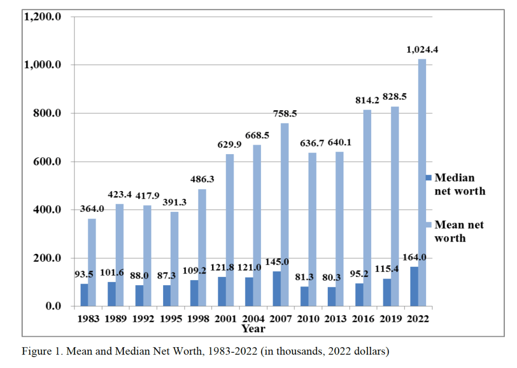
Wolff uses data from the Federal Reserve’s Survey of Consumer Finances to measure the wealth, or net worth, of people in these age groups—the market value of their financial assets minus the market value of their financial liabilities. He includes in his measure of assets the market value of people’s real estate holdings—including their homes—stocks and bonds, bank deposits, contributions to defined contribution pension funds, unincorporated businesses, and trust funds. He includes in his measure of liabilities people’s mortgage debt, consumer debt—including credit card balances—and other debt, such as educational loans. Because Wolff wants to focus on that part of wealth that is available to be spent on consumption, he refers to it as financial resources, and he excludes from his wealth measure the present value of future Social Security payments and the present value of future defined contribution pension benefits.
The following figure from Wolff’s paper shows that, using his definition, both median and mean wealth have increased substantially from 1987 to 2o22. Note that both measures of average wealth declined during the Great Recession and Global Financial Crisis of 2007–2009. Median wealth declined by nearly 44 percent between 2007 and 2010. That median wealth grew much faster than mean wealth over the whole period indicates that wealth inequality.
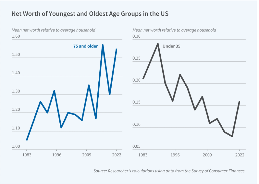
Although the average wealth of all age groups increased over this period, the relative wealth of households 75 years and older rose and the relative wealth of households 35 years and younger fell. The following figure from the NBER Digest illustrates this shift. The 75 and over age group increased its mean net worth from 5 percent greater than the mean net worth of the average household in 1983 to 55 percent of the mean net worth of the average household in 2022. In contrast, the 35 and under age group saw its mean new worth relative to the average household fall from 21 percent in 1983 to 16 percent in 2022. Note, though, that there is significant volatility over time in the relative wealth shares of the two age groups.
What explains the relative increase in wealth among households 75 and over and the relative decrease in wealth among households 35 and under? Wolff identifies three key factors:
“[T]he homeownership rate, total stocks directly and indirectly owned, and home mortgage debt. The homeownership rate is the same in the two years for the youngest group but falls relative to the overall rate, whereas it shoots up for the oldest group both in actual level and relative to the overall average. The value of stock holdings rises for both age groups but vastly more for the oldest households compared to the youngest ones and accounts for a substantial portion of the elderly’s relative wealth gains. Mortgage debt rises in dollar terms for both groups but considerably more in relative terms for the youngest group.”
Perhaps surprisingly, Wolff finds that “despite dire press reports, educational loans fail to appear as a significant factor” in explaining the decline in the relative wealth of younger households.
Glenn, along with co-authors Douglas Elmendorf of Harvard’s Kennedy School and Zachary Liscow of the Yale Law School, has written a new National Bureau of Economic Research working paper: “Policies to Reduce Federal Budget Deficits by Increasing Economic Growth”
Here’s the abstract:
Could policy changes boost economic growth enough and at a low enough cost to meaningfully reduce federal budget deficits? We assess seven areas of economic policy: immigration of high-skilled workers, housing regulation, safety net programs, regulation of electricity transmission, government support for research and development, tax policy related to business investment, and permitting of infrastructure construction. We find that growth-enhancing policies almost certainly cannot stabilize federal debt on their own, but that such policies can reduce the explicit tax hikes, spending cuts, or both that are needed to stabilize debt. We also find a dearth of research on the likely impacts of potential growth-enhancing policies and on ways to design such policies to restrain federal debt, and we offer suggestions for ways to build a larger base of evidence.
The economy and financial markets nervously await the July 8 end of the 90-day pause of the Trump administration’s “reciprocal” tariffs. But four days earlier, Republicans can allay those fears with a pro-growth policy that advances President Trump’s Made in America agenda without tariffs. The fix: tax reform.
July 4 is the date that Treasury Secretary Bessent has predicted Congress and the White House will have ready a 2.0 version of the landmark Tax Cut and Jobs Act of 2017, or TCJA. Without congressional action, some of these reforms will expire at the end of 2025, killing changes that still benefit the economy. Corporate tax changes, in particular, boosted investment and growth. These should remain the focal point of this next tax bill—for many reasons. Done right, corporate tax reform could advance President Trump’s goal to bring investment to American production without using economy-roiling tariffs. Call it TCJA+.
Renewing some parts of the original TCJA will help investment in the U.S. The 2017 reform offered incentives for investment in new businesses by allowing them to expense the cost of assets, rather than writing them off over time. But these benefits were set to be phased out from 2023 to 2026, removing a key pro-growth element of the earlier law.
Then there are two new provisions Republicans should add to secure Mr. Trump’s goal to have more made in America. Both were in the original 2016 House Republican tax reform blueprint.
First, Congress should change business taxation from the current income tax to a cash-flow tax, which taxes a firm’s revenue, minus all its expenses, including investment. Long championed by economists and tax-law experts, a cash-flow tax would allow businesses to expense investment immediately. It would also disallow nonfinancial companies from making interest deductions, because unlike an income tax, a cash-flow tax treats debt and equity the same. This removes an important tax incentive for firms to allow themselves to be leveraged. A cash-flow tax is also much simpler than a corporate income tax, which requires complex depreciation schedules. Most important, the reform would stimulate business investment.
Second, legislators should add a border adjustment to corporate taxes. That would deny companies a tax deduction for expenses of inputs imported from abroad, while exempting U.S. exports from taxation. As the Trump administration has observed, other countries already use border adjustments in their value-added taxes on consumption. America uses a similar mechanism in state and local retail taxes, too. If you buy a kitchen appliance in New York, you pay New York sales tax, even if it was made in Ohio. Sales tax applies only where the good is sold, not where it originates.
Though distinct from tariffs, border adjustments can promote domestic production. Adding a border adjustment to the federal corporate tax would eliminate any extra tax businesses suffer now simply as a consequence of producing in the U.S. Though the 2017 law made the U.S. tax system more globally competitive by lowering the corporate income tax rate from 35% to 21%, it’s still higher than in many other countries, which attract production with low cost. A border adjustment would remove this incentive for American firms to locate profits or activities abroad, while increasing incentives for non-U.S. firms to locate activities within our borders.
As with the original pro-investment features in the 2017 law, this TCJA+ reform would increase investment and incomes—and thereby revenue. For the original TCJA, when the Congressional Budget Office included the macroeconomic effects of higher incomes buoyed by the reforms’ pro-growth elements, the CBO reduced the estimated revenue loss from the tax cuts by almost 30%. Changing the corporate income tax to a cash-flow levy would similarly increase revenue by removing taxes on what economists call the “normal return” on investment, or the cost of capital. Companies would instead pay only on profits above this amount. A border adjustment can likewise raise substantial revenue over the next decade because imports (which would receive no deduction) are larger than exports (which would no longer be taxed).
The higher revenue these two TCJA+ provisions promise could be used to lower the tax rate on business cash flow or to fund other tax-policy objectives. Importantly, that revenue can replace revenue raised from the tariffs the Trump administration had planned to implement on July 8. These two tax provisions would accomplish the president’s America-first and revenue objectives without destabilizing businesses with whipsawing tariffs.
Finally, TCJA+ would offer another big benefit: It would move the U.S. toward independence from political meddling in the economy via targeted protection or subsidies. This added predictability and breathing room for investment would be one more reason to produce in America. Pluses indeed.
Logo of the Congressional Budget Office from cbo.gov.
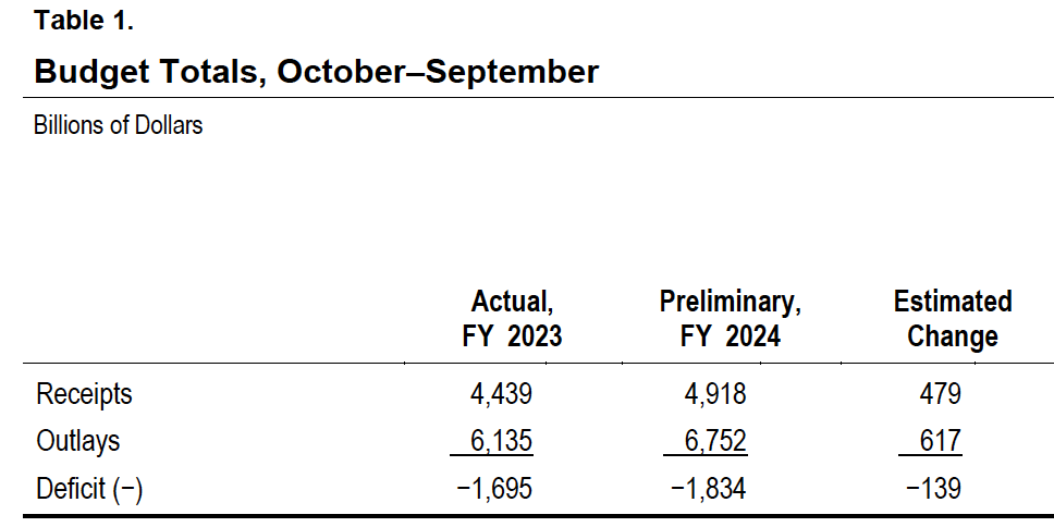
The federal government’s fiscal year runs from October 1 to September 30 of the following calendar year. The Congressional Budget Office (CBO) estimates that the federal government’s budget deficit for fiscal 2024, which just ended, was $1.8 trillion. (The Office of Management and Budget (OMB) will release the official data on the budget later this month.)
The federal budget deficit increased by about $100 billion from fiscal 2023, although the comparison of the deficits in the two years is complicated by the question of how to account for the $333 billion in student debt cancellation that President Biden ordered (which would reduce federal revenues by that amount) but which wasn’t implemented because of a decision by the U.S. Supreme Court.
The following table from the CBO report compares federal receipts and outlays for fiscal years 2023 and 2024. Recipts increased by $479 billion from 2023 to 2024, but outlays increased by $617 billion, resulting in an increase of $139 billion in the federal budget deficit.
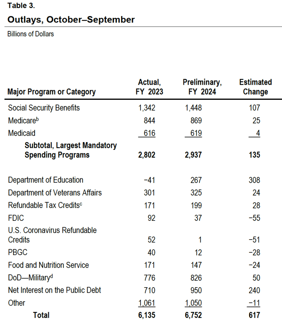
The following table shows the increases in the major spending categories in the federal budget. Spending on the Social Security, Medicare, and Medicaid programs increased by a total of $135 billion. The large increase in spending on the Department of Education is distorted by accounting for the reversal of the student debt cancellation following a Suprement Court ruling, as previously mentioned. The FDIC is the Federal Deposit Insurance Corporation, which had larger than normal expenditures in 2023 due the failure of several regional banks. (We discuss this episode in several earlier blog posts, including this one.) Interest on the public debt increased by $240 billion because of increases in the debt as a result of persistently high federal deficits and because of increases in the interest rates the Treasury has paid on new issues of bill, notes, and bonds necessary to fund those deficits. (We discuss the federal budget deficit and federal debt in Macroeconomics, Chapter 16, Section 16.6 (Economics, Chapter 26, Section 26.6).)
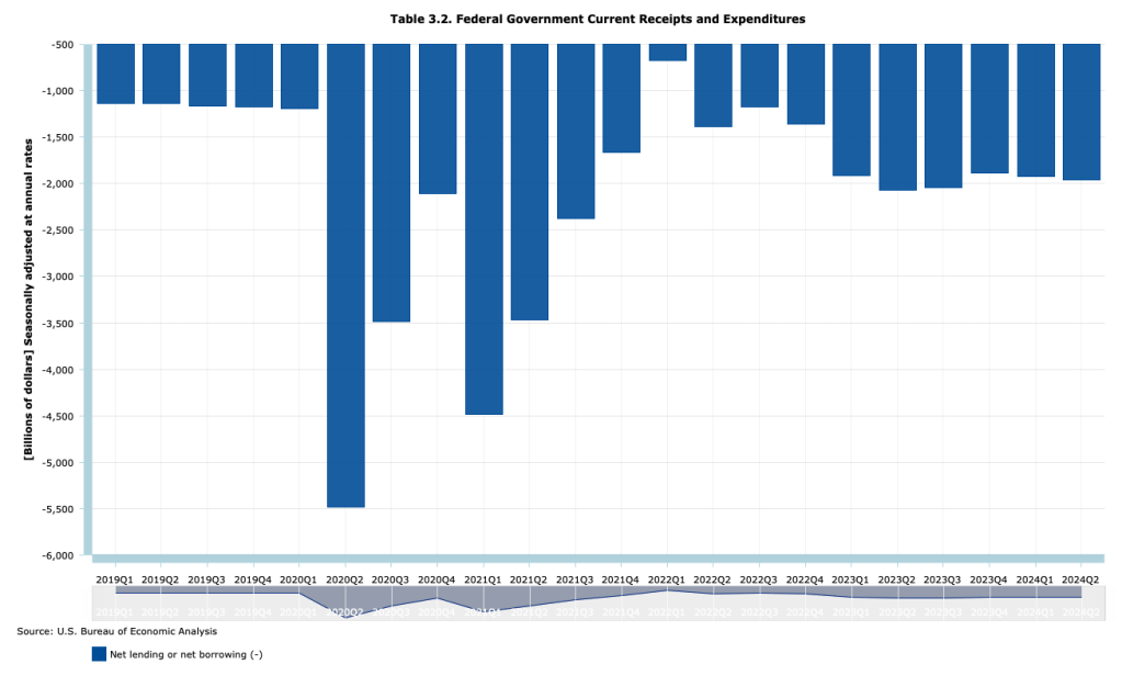
A troubling aspect of the large federal budget deficits is that they are occurring during a time of economic expansion when the economy is at full employment. The following figure, using data from the Bureau of Economic Analysis (BEA), shows that at an annual rate, the federal budget deficit has beening running between $1.9 trillion and $2.1 trillion each quarter since the first quarter of 2023, well after most of the federal spending increases to meet the Covid pandemic ended.
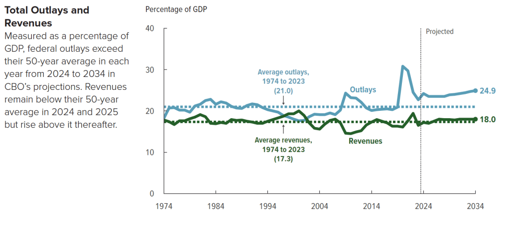
The following figure from the CBO shows trends in federal revenue and spending. From 1974 to 2023, federal spending averaged 21.o percent of GDP, but is forecast to rise to 24.9 percent of GDP by 2023. Federal revenue averaged 17.3 percent of GDP from 1974 to 2023 and is forecast to rise to 18.0 percent of GDP in 2034. As a result, the federal budget deficit, which had averaged 3.7 percent of GDP between 1974 and 2023 (already high in a longer historical context) will nearly double to 6.9 percent of GDP in 2034.
Slowing the growth of federal spending may prove difficult politically because the majority of spending increases are from manadatory spending on Social Security and Medicare, and from interest on the debt. Discretionary outlays are scheduled to decline in future years according to current law, but may well also increase if Congress and future presidents increase defense spending to meet the foreign challenges the country faces.
One possible course of future policy that would result in smaller future federal deficits is outlined in this post and the material at the included links.
Glenn serves on the the Grand Bargain Committee, chaired by Michael Strain of the American Enterprise Institute and Isabel Sawhill of the Brookings Institution. The committee, whose members span the political spectrum, have prepared a report that addresses some of the country’s most pressing economic and social problems.
Glenn and Michael Strain prepared the following introduction to the report. Below there is a link to the whole report.
The views expressed in this report are those of the individual authors who collectively constitute the Grand Bargain Committee, co-chaired by Michael R. Strain and Isabel V. Sawhill. This report was sponsored by the Center for Collaborative Democracy and was prepared independent of influence from the center and from any other outside party or institution. It is being published by the Bipartisan Policy Center as an example of how people with diverse views and political leanings can find common ground. The recommendations are strictly those of the policy experts and do not necessarily reflect the views of any organization or those of the BPC. All data are current as of November 2023.
By: Eric Hanushek, G. William Hoagland, Douglas Holtz-Eakin, R. Glenn Hubbard, Maya MacGuineas, Richard V. Reeves, Robert D. Resichauer, Gerard Robinson, Isabel V. Sawhill, Diane Schanzenbach, Richard Schmalensee, Michael R. Strain, and C. Eugene Steuerle.
Introduction
The United States faces serious economic and social challenges, including:
The underlying economic growth rate has slowed, as have opportunities for people to move up the economic ladder.
Our education system fails too many children and leaves many more with fewer opportunities than they deserve.
The nation is not rising to the challenge of addressing climate change.
Both our health care system and the health of our population need improvement.
Our income tax system is broken, generating tax revenue in an inefficient and unfair manner.
And the national debt is growing at an unsustainable pace, threatening long-term economic growth, crowding out needed investments in economic opportunity, and placing the nation’s ability to respond to a future crisis at risk.
To address these problems, the Center for Collaborative Democracy commissioned subject matter experts—progressives, centrists, and conservatives—to develop a “Grand Bargain” encompassing all six issues. The policy debate typically puts these problems into silos, and within each silo, powerful forces support the status quo. This report seeks to break down these silos. Dealing with them all at once—in a Grand Bargain—is a more promising strategy than dealing with them individually, because it allows for different parties to strike deals across policy issues, not just within a single issue.
For example, implementing a carbon tax to address climate change seems impossibly difficult. So does increasing accountability for teacher performance. Trading one for the other might be easier than pursuing both in isolation. Fixing the structural budget deficit by reducing entitlement spending is an enormous political challenge. So is increasing spending on programs that advance economic opportunity. Doing both at the same time could be more politically feasible than addressing them separately.
In this context, the group of experts met for several months in 2023 to share perspectives and ideas and to come up with sensible policies in each of these areas: economic growth and mobility; education; environment; health; taxes; and the federal budget. The end result is this report, which is being published by the Bipartisan Policy Center as an example of how people with diverse views and political leanings can find common ground.
This report is short, consisting of less than 30 pages of text. Its brevity is by design. This constraint forced the group to stay focused on issues and recommendations that matter the most. The focus of the report is on concepts. It is designed to answer such questions as, “How should the nation’s approach to education or to the federal budget change? What fundamental reforms are required to increase the underlying rates of economic growth and upward mobility?” Focusing on concepts means not focusing on policy details, including the details of implementing our recommendations and of transitioning across policy regimes. Our lack of attention to policy details does not mean we do not recognize their importance. Of course, we do, and many members of the group have spent much of their careers studying and designing public policies. Instead, we focus on concepts because we believe the United States needs to return to a discussion of first principles. This report advances that objective.
Not every member of the group agrees with every recommendation in this report. That is not surprising given the diversity of views in the group, and the difficulty and complexity of many of the issues we address. Despite this disagreement, we were able to have an informed and constructive discussion about these economic issues, to find compromises, and to come up with a set of recommendations that we believe, on balance, would greatly strengthen the country and improve people’s lives.
We believe in the importance of a market economy. Free markets have led to unprecedented growth and innovation, along with rising incomes, over the past three centuries. But government also has a role to play. To unleash more growth, we need to curtail unneeded or overly costly regulations and to create a tax system that encourages investment spending and innovation. To bring prosperity to more people, we need policies that will enable more people to benefit from economic growth through investment in their education and skills. For this reason, we put a great deal of emphasis on improving education for children, on training or retraining for adult workers, and on subsidizing the earnings of low-wage workers when necessary while maintaining a safety net for those who cannot work.
Our proposals are designed to advance certain underlying values and themes: Work and savings should be rewarded, investment should be encouraged over consumption, public assistance should be better targeted to those most in need, the tax system should be more progressive, and the nation should invest relatively more in the young and spend relatively less on the elderly.
Our specific proposals in each area are as follows:
On economic growth and mobility, we recommend investing in the education and training of workers, through community colleges and apprenticeships. We call for a more skill-based immigration system and for more immigrants; for encouraging innovation by investing more in basic research; for reducing taxes on new investment; for curbing unneeded regulation; for reducing the national debt; and for encouraging participation in economic life by increasing the generosity of earnings subsidies for low-wage workers.
On education, we recommend improving the teacher workforce at the K-12 level; paying teachers more but strengthening the link between pay and performance; maintaining educational standards and accountability while narrowing gaps by race and class; expanding school choice; and recognizing the role that parents and families must play in students’ learning.
On the environment, our main recommendation is to adopt a carbon tax. We also call for reducing methane emissions; expanding federal authority in the planning, siting, and permitting of the national electric transmission system; and repealing the renewable fuel standard that requires refiners to blend corn ethanol into the fuel they sell.
On health, we call for giving more attention to the social determinants of poor health with a focus on the need for better nutrition, for rationalizing existing subsidies for health care, and for reducing health care costs.
On taxes, we call for increasing tax revenue as a share of annual gross domestic product (GDP), and for that revenue to be raised in a manner that is more progressive, efficient, and simple than under current law, while also increasing the incentive to save and invest. For the business sector, that means allowing the expensing of investment expenditures and moving toward equal treatment of the corporate and noncorporate sectors.
On the federal budget, we recommend putting the debt as a share of annual GDP on a sustainable trajectory with a comprehensive package of reforms made up of a rough balance between tax increases and spending cuts in the initial years, phasing into a much larger share of the savings coming from spending cuts over time.
Most of these recommendations are at the federal level, but some are at the state and local level, particularly our education recommendations.
In the spirit of a Grand Bargain, these recommendations advance common goals and values through compromises both within and across policy areas. For example, one of our values is reflected in the goal of refocusing government spending on those who truly need it, and another is to restore fiscal responsibility. To accomplish this, we call for slower growth in Social Security and Medicare benefits for affluent seniors to reduce the major driver of the national debt, but we also protect vulnerable seniors and spend more on the education of children and on earnings subsidies for the working poor. We recommend adopting a carbon tax because it will simultaneously advance our goals of supporting the environment, increasing tax revenue, and boosting dynamism by encouraging innovation in the energy sector.
We believe the analysis and recommendations in this report point a path forward for the nation, but we offer them in a spirit of humility, understanding that others will disagree. We hope that this report catalyzes a much needed debate about the future of our nation.
President Lyndon Johnson signing the Economic Opportunity Act in 1964. (Photo from Wikipedia)
In 1964, President Lyndon Johnson announced that the federal government would launch a “War on Povery.” In 1988, President Ronald Regan remarked that “some years ago, the Federal Government declared war on poverty, and poverty won.” Regan was exaggerating because, however you measure poverty, it has declined substantially since 1964, although the official poverty rate has remained stubbornly high since the early 1970s.
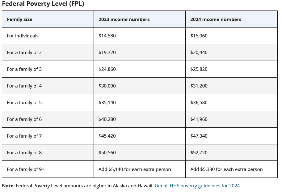
Each year the U.S. Census Bureau calculates the official poverty rate—the fraction of the population with incomes below the federal poverty level, often called the poverty line. The following table shows the poverty line for the years 2023 and 2024 illustrating how it varies with the size of a household:
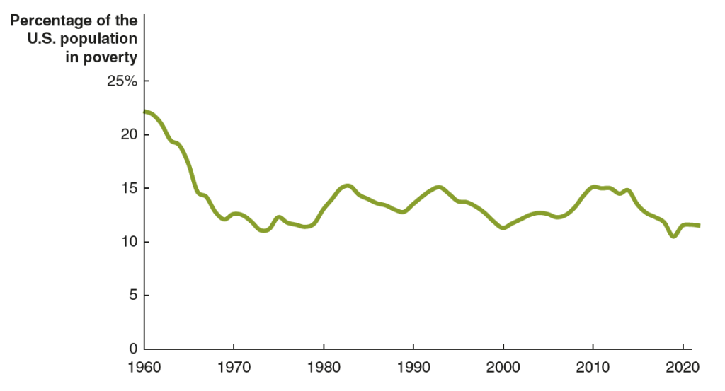
The following figure shows the official poverty rate for the years from 1960 to 2022. The poverty rate in 1960 was 22.2 percent. By 1973, it had been cut in half to 11.1 percent. The decline in the poverty rate largely stopped at that point. In the following years the official poverty rate fluctuated but stopped trending down. In 2022, the poverty rate was 11.5 percent—actually higher than in 1973. (The Census Bureau will release the poverty rate for 2023 later this month.)
But is the official poverty rate the best way to measure poverty? In Microeconomics, Chapter 17, Section 17.4 (Economics, Chapter 27, Section 27.4), we discuss some of the issues involved in measuring poverty. One key issue is how income should be measured for purposes of calculating the poverty rate. In an academic paper, Richard Burkhauser, of the University of Texas, Kevin Corinth, of the American Enterprise Institute, James Elwell, of the Congressional Joint Committee on Taxastion, and Jeff Larimore, of the Federal Reserve Board, carefully consider this issue. (The paper can be found here, although you may need a subscription or access through your library.)
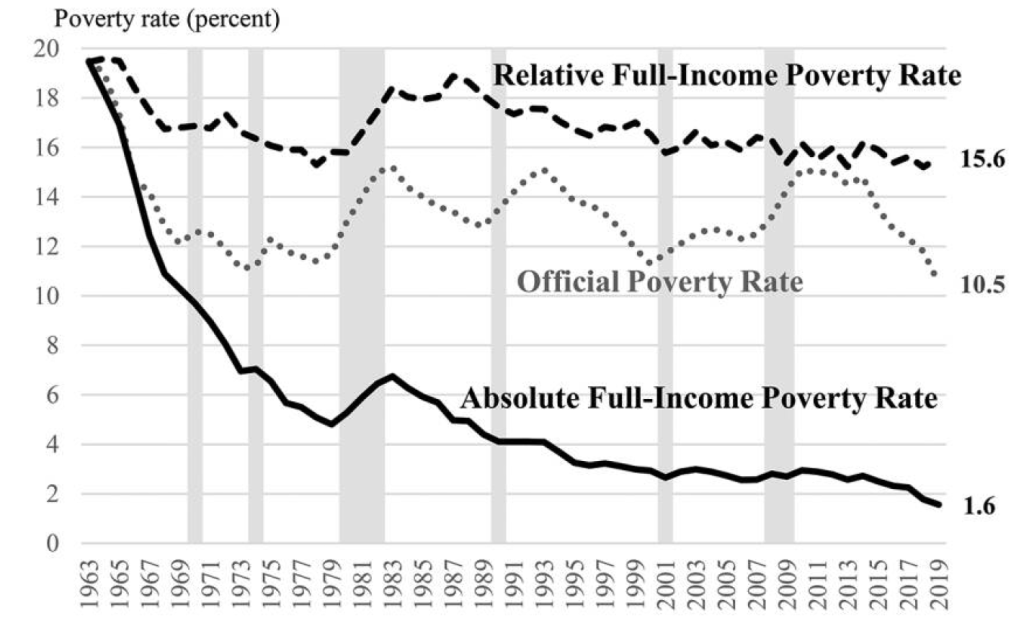
They find that using an adjusted measure of the poverty line and a fuller measure of income results in the poverty rate falling from 19.5 percent in 1963 to 1.9 percent in 2019. In other words, rather than the poverty rate stagnating at around 11 percent—as indicated using the official poverty numbers—it actually fell dramatically. Rather than progress in the War on Poverty having stopped in the early 1970s, these results indicate that the war has largely been won. The authors, though, provide some important qualifications to this conclusion, including the fact that even 1.9 percent of the population represents millions of people.
Discussions of poverty distinguish between absolute poverty—the ability of a person or family to buy essential goods and services—and relative poverty—the ability to buy goods and services similar to those that can be purchased by individuals and families with the median income. The authors of this study argue that in launching the War on Povery, President Johnson intended to combat absolute poverty. Therefore, the authors start with the poverty line as it was in 1963 and increase the line each year by the rate of inflation, as measured by changes in the personal consumption expenditures (PCE) price index.
To calculate what they call “the absolute full-income poverty measure (FPM)” they include in income both cash income and “in-kind programs designed to fight poverty, including food stamps (now the Supplemental Nutrition Assistance Program [SNAP]), the schoollunch program, housing assistance, and health insurance.” As noted earlier, using this new definition, the overall poverty rate declined from 19.5 percent in 1963 to 1.9 percent in 2019. The Black poverty rate declined from 50.8 percent in 1963 to 2.9 percent in 2019.
The author’s find that the War on Poverty has been less successful in reducing relative poverty. Linking increases in the poverty line to increases in median income results in the poverty rate having decreased only from 19.5 percent in 1963 to 15.6 percent in 2019. The authors also note that not as much progress has been made in fulfilling President Johnson’s intention that: “The War on Poverty is not a struggle simply to support people, to make them dependent on the generosity of others.” They find that the fraction of working-age people who receive less than half their income from working has increased from 4.7 percent in 1967 to 11.0 percent in 2019.
The following figure from the authors’ paper shows the offical poverty rate, the absolute full-income poverty rate—which the authors believe does the best job of representing President Johnson’s intentions when he launched the War on Poverty—and the relative poverty rate.
Because of disagreements on how to define poverty and because of the difficulty of constructing comprehensive measures of income—difficulties that the authors discuss at length in the paper—this paper won’t be the last word in assessing the results of the War on Poverty. But the paper provides an important new discussion of the issues involved in measuring poverty.
Image of servers in a restaurant generated by ChatGTP-4o.
How should you track over time the real wagees of low-wage workers? If you are interested in income mobility, you would want to track the experience over the course of their working lives of individuals who began their careers in low-wage occupations. Doing so would allow you to measure how well (or poorly) the U.S. economy succeeds in providing individuals with opportunities to improve their incomes over time.
You might also be interested in how the real wages of people who earn low wages has changed over time. In this case, rather than tracing the wages over time of individuals who earn low wages when they first enter the labor market, you would look at the real wages of people who earn low wages at any given time. The simplest way to do that analysis would be using data on the average nominal wage earned by, say, the lowest 20 percent of wage earners, and deflate the average nominal wage by a price index to determine the average real wage of these workers. How the average real wage of low-wage workers varies over time provides some insight into the changing standard of living of low-wage workers.
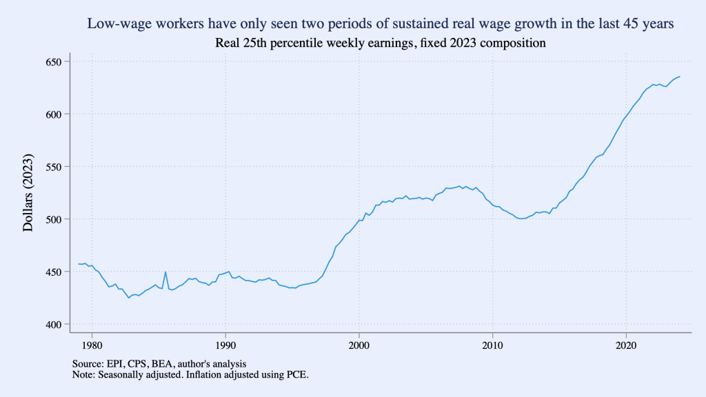
In a recent Substack post, Ernie Tedeschi, Director of Economics at the Budget Lab research center at Yale University, has carried out a careful analysis of movements over time in the average real wage of low-wage workers. Tedeschi points out a complicating factor in this analysis: “The population has gotten older over time and more educated. The workforce looks different too, with more workers in services and fewer in manufacturing. Shifting populations means that comparisons of workers aren’t apples-to-apples over time.”
To correct for these confounding factors, Tedeschi constructs a low-wage index that makes it possible to examine the real wage of low-wage workers, holding constant the composition of low-wage workers with respect to “sex, age, race, college education, and broad industry and occupation” at the values of these characteristics in 2023. Using this approach, makes it possible to separate changes in wages of workers with given characteristics from changes in wages that occur because the average characteristics of workers has changed. For example, on average, workers who are older or who have more years of education will be more productive and, therefore, on average will earn higher wages than will workers who are younger or have fewer years of education.
The following figure from Tedeschi’sSubstack post shows movements in his low-wage index during each quarter from the first quarter of 1979 to the first quarter of 2024, with “low wage” defined as workers at the 25th precentile of the distribution of wages. (That is, 24 percent of workers receive lower wages and 75 percent of workers receive higher wages than do these workers.) The index shows that a low-wage worker in 2024 has a much higher real wage than a low-wage worker in 1979, but the increase in the average real wage occurs mainly during two periods: 1997–2007 and 2014–2024. (Tedeschi uses the person consumption expenditures (PCE) price index to convert nominal wages to real wages.)
A more complete discussion of Tedeschi’s methods and results can be found in his blog post.
Supports: Microeconomics and Economics, Chapter 6.
Photo from the New York Times.
Blogger Matthew Yglesias made the following observation in a recent post: “If you look at gasoline prices, it’s obvious that if fuel gets way more expensive next week, most people are just going to have to pay up. But if you compare the US versus Europe, it’s also obvious that the structurally higher price of gasoline over there makes a massive difference: They have lower rates of car ownership, drive smaller cars, and have a higher rate of EV adoption.” (The blog post can be found here, but may require a subscription.)
What does Yglesias mean by Europe having a “structurally higher price” of gasoline?
Assuming Yglesias’s observations are correct, what can we conclude about the price elasticity of the demand for gasoline in the short run and in the long run?
Currently, the federal government imposes a tax of 18.4 cents per gallon of gasoline. Suppose that Congress increases the gasoline tax to 28.4 cents per gallon. Again assuming that Yglesias’s observations are correct, would you expect that the incidence of the tax would be different in the long run than in the short run? Briefly explain.
Would you expect the federal government to collect more revenue as a result of the 10 cent increase in the gasoline tax in the short run or in the long run? Briefly explain.
Solving the Problem
Step 1: Review the chapter material. This problem is about the determinants of the price elasticity of demand and the effect of the value of the price elasticity of demand on the incidence of a tax, so you may want to review Chapter 6, Section 6.2 and Solved Problem 6.5. (Note that a fuller discussion of the effect of the price elasticity of demand on tax incidence appears in Chapter 17, Section 17.3.)
Step 2: Answer part a. by explaining what Yglesias means when he writes that Europe has a “structurally higher” price of gasoline. Judging from the context, Yglesias is saying that European gasoline prices are not just temporarily higher than U.S. gasoline prices but have been higher over the long run.
Step 3: Answer part b. by expalining what we can conclude from Yglesias’s observations about the price elasticity of demand for gasoline in the short run and in the long run. When Yeglesias is referring to gasoline prices rising “next week,” he is referring to the short run. In that situation he says “most people are going to have to pay up.” In other words, the increase in price will lead to only a small decrease in the quantity demanded, which means that in the short run, the demand for gasoline is price inelastic—the percentage change in the quantity demanded will be smaller than the percentage change in the price.
Because he refers to high gasoline prices in Europe being structural, or high for a long period, he is referring to the long run. He notes that in Europe people have responded to high gasoline prices by owning fewer cars, owning smaller cars, and owning more EVs (electric vehicles) than is true in the United States. Each of these choices by European consumers results in their buying much less gasoline as a result of the increase in gasoline prices. As a result, in the long run the demand for gasoline is price elastic—the percentage change in the quantity demanded will be greater than the percentage change in the price.
Note that these results are consistent with the discussion in Chapter 6 that the more time that passes, the more price elastic the demand for a product becomes.
Step 4: Answer part c. by explaining how the incidence of the gasoline tax will be different in the long run than in the short run. Recall that tax incidence refers to the actual division of the burden of a tax between buyers and sellers in a market. As the figure in Solved Problem 6.5 illustrates, a tax will result in a larger increase in the price that consumers pay for a product in the situation when demand is price inelastic than when demand is price elastic. The larger the increase in the price that consumers pay, the larger the share of the burden of the tax that consumers bear. So, we can conclude that the tax incidence of the gasoline tax will be different in the short run than in the long run: In the short run, more of the burden of the tax is borne by consumers (and less of the burden is borne by suppliers); in the long run, less of the burden of the tax is borne by consumers (and more of the burden is borne by suppliers).
Step 5: Answer part d. by explaining whether you would expect the federal government to collect more revenue as a result of the 10 cent increase in the gasoline tax in the short run or in the long run. The revenue the federal government collects is equal to the 10 cent tax multiplied by the quantity of gallons sold. As the figure in Solved Problem 6.5 illustrates, a tax will result in a smaller decrease in the quantity demanded when demand is price inelastic than when demand is price elastic. Therefore, we would expect that the federal government will collect more revenue from the tax in the short run than in the long run.
Photo from the Associated Press via the Wall Street Journal.
A tax is progressive if people with lower incomes pay a lower percentage of their income in tax than do people with higher incomes. (We discuss the U.S. tax system in Microeconomics and Economics, Chapter 17, Section 17.2.) Recently, the Joint Committee on Taxation (JCT) of the U.S. Congress released a report, “Overview of the Federal Tax System as in Effect for 2024,” that provides data on the progressivity of the U.S. tax system. (An overview of the role of the JCT can be found here.)
The progressivity of the federal individual income tax is shown in the following figure from the JCT report. The column on the right shows that for each category of taxpayers shown—single people, heads of households (who are unmarried people who financially support at least one other person), and married people—the marginal income tax rate increases with a taxpayer’s income. The marginal tax rate is the rate that someone pays on additional income that they earn. So, for instance, the table shows that an individual who has taxable income of $80,000 faces a marginal tax rate of 22 percent because that is the rate the person pays on the income they earn between $47,150 and $80,000. An individual who has a taxable income of $700,000 faces a marginal tax rate of 37 percent because that is the rate the person pays on the income they earn between $609,350 and $700,000.
In Chapter 17, we use data from the Tax Policy Center to show the average income tax rate paid by different income groups. The average tax rate is computed as the total tax paid divided by taxable income. The marginal tax rate is a better indicator than the average tax rate of how a change in a tax will affect a person’s willingness to work, save, and invest. For instance, if you are considering working more hours in your job or taking on a second job, such driving part time for Uber or Lyft, you want to know what your tax rate is on the additional income you will earn. For that purpose, you should ignore your average tax rate and instead focus on your marginal tax rate.
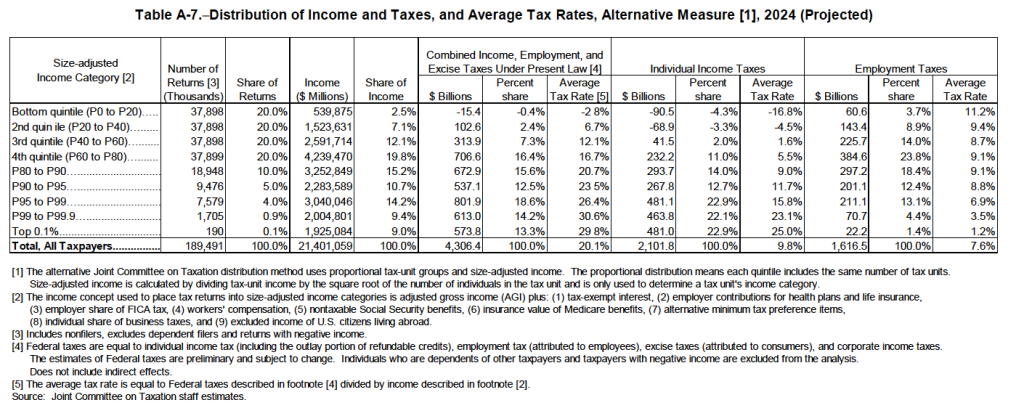
The following table from the JCT report is similar to the table in Chapter 17, which was based on data from the Tax Policy Center. The JCT report has the advantage of direct access to government tax data, which, as a private group, the Tax Policy Center doesn’t have. In addition, the JCT reports on an income group—the top 0.1 percent of income earners—compiled from government data not available to the Tax Policy Center. (Much political discussion has focused on the income earned and taxes paid by the top 1 percent of earners, which is a much larger group than the top 0.1 percent. We discuss the top 1 percent in the Apply the Concept, “Who Are the 1 Percent, and How Do They Earn Their Incomes,” in Microeconomics and Economics, Chaper 17, Section 17.4.)
The table shows data for the first four quntiles (or groups of 20 percent of taxpayers), with the highest quintile divided further. The table shows that the federal individual income tax is highly progressive, with the two lowest income quintiles having negative average tax rates because they receive more in tax credits than they pay in taxes. Employment taxes—primarily the payroll tax used to fund the Social Security and Medicare Systems—are regressive, with the lowest deciles paying a larger percentage of their income in these taxes than do the higher deciles. The regressivity of employment taxes is the result of both payroll taxes being levied on the first dollar of wages and salaries individuals earn and the part of the payroll tax used to fund the Social Security system dropping to zero for incomes above a certain level—$168,600 in 2024. Because income taxes are much larger in total than employment taxes or excise taxes—such as the federal taxes on gasoline, airline tickets, and alcoholic beverages—the total of these three types of federal taxes is progressive, as shown by the fact that the average tax rate rises with income. (Although note that the top 0.1 percent pay taxes at a slightly lower rate than do the other taxpayers included in the top 1 percent.)