AI on the AI Revolution

Image created by ChatGPT, as are the other images in this post.

Technological breakthroughs are often embodied in machinery, equipment, or, as in the case of artificial intelligence (AI), software. For example, the Industrial Revolution of the late 1700s, which involved mass production of low-priced cotton textiles, was made possible by the development in England of large cotton spinning machines that were often powered by steam engines. 

Other technological breakthroughs are disembodied because they involve reorganizing production rather than employing new machinery or software. For example, the just-in-time (JIT) system that Toyota developed beginning in the 1940s, lowered the costs of assembling automobiles by, among other things, having parts arrive at a factory just when needed.

Across U.S. history, there have been a number of technological revolutions that required massive capital investments.  For instance, the transportation revolution of the early 1800s that significantly reduced the costs of shipping freight, relied on substantial investments in canals.  Later in the 1800s, transportation costs were reduced further as firms invested in the largest network of railroads in the world. Electrification of businesses and private homes in the late 1800s and early 1900s required the building of power plants and transmission lines. In the late 1990s, many firms competed to build networks of fiber-optic cable to carry the rapid increase in digital traffic resulting from the development of the internet.

Each of these technological revolutions succeeded in providing consumers with new or lower-cost goods or services. But building the physical capital that embodied these technologies could result in substantial losses or bankruptcy. For example, in the 1830s, several states, including Pennsylvania, Illinois, and Michigan, defaulted on the bonds they had issued to finance canal instruction.

Similarly, in the 1890s, some of the largest private railroad companies in the United States, including the Union Pacific, the Northern Pacific, and the Atchison, Topeka & Santa Fe, went bankrupt. In the early 2000, investors realized that internet commerce wouldn’t expand as rapidly as they had expected. As a result, several prominent internet firms, such as Pets.com and eToys.com, saw their stock prices collapse in what was called the dot com crash, and eventually declared bankruptcy.  Several firms that had invested in building large fiber-optic networks, including Worldcom and Global Crossing, also failed.

Why did the companies making large capital investments in new technologies sometimes fail even though the technologies themselves proved to be revolutionary? The answer in part is that forecasting accurately the demand for a new product can be difficult. For example, ultimately the level of internet traffic was more than great enough to justify the investment in fiber-optic networks, but the increase came too late for some companies to avoid bankruptcy. Competition among firms to take advantage of a new technology can lead to overbuilding, as when railroad companies built more miles of track than were needed to meet the demand to transport freight and passengers.

A number of economists and investment analysts have noted that the very heavy investment in data centers used to power AI models resembles the large capital investments firms made during earlier technological revolutions. As the following figure shows, beginning in early 2023, shortly after the public release of ChatGPT, the first widely used AI chatbot, investment in information processing equipment and software as a percentage of all nonresidential fixed investment has increased dramatically.

Do the firms building data centers run the risk of overestimating demand for AI and overbuilding data centers? More generally, how does the build-out of AI data centers compare with the earlier build-outs of railroads and fiber-optic networks? Who better to answer this question than ChatGPT!

The following (very long!) answer was ChatGPT’s response to the following prompt: “In what ways is the current build-out of AI data centers similar to the build-out of the railroad network in the United States in the late nineteenth century and the build-out of the fiber-optic network in the United States in the 1990s and in what ways is it different?” (A quick summary is given in the brief “Bottom Line” section at the very end.)

AI Data Centers, Railroads, and Fiber-Optic Networks

The best way to frame the comparison is this:

The railroad analogy is most useful for understanding the physical scale, bottlenecks, public subsidies, and geographic consequences of the AI buildout. The fiber-optic analogy is most useful for understanding its financial risks, uncertain demand, rapid technological improvement, and potential for overcapacity.

AI data centers nevertheless differ importantly from both. They are not simply links in a transportation or communications network. They are more like factories that produce computing services, and the extremely expensive machinery inside them becomes obsolete much faster than either railroad rights-of-way or buried fiber.

The scale is already extraordinary. The International Energy Agency estimates that the largest technology companies spent more than $400 billion on capital investment in 2025 and expects that figure to rise about 75 percent in 2026. U.S. data centers consumed approximately 176 terawatt-hours of electricity in 2023—4.4 percent of U.S. electricity use—and Berkeley Lab projects consumption of 325–580 terawatt-hours by 2028.

Ways the three buildouts are similar

1. All three are investments in enabling infrastructure

Railroads did much more than generate revenue from tickets and freight charges. They brought previously isolated regions into a national market, encouraged settlement, changed the location of factories and cities, and made complementary investments in farms, mines, warehouses, and factories more valuable. The United States added roughly 170,000 miles of railroad track between 1871 and 1900. 

Fiber-optic builders similarly expected abundant bandwidth to generate applications that could not yet be foreseen. More bandwidth would encourage new internet services, which would increase bandwidth demand, which would justify still more fiber.

The AI argument is nearly identical: companies are building computing capacity before all its profitable applications have been discovered. The value of the data centers will depend partly on complementary developments—better models, proprietary data, new software, organizational changes, and the willingness of companies and consumers to pay for AI services.

In all three cases, therefore, infrastructure and applications are jointly determined. Waiting until demand is plainly visible can mean waiting too long, because the infrastructure itself helps create the demand.

2. High fixed costs encourage companies to build ahead of demand

A railroad requires land, grading, bridges, tunnels, stations, track, and rolling stock before it carries its first paying customer. A fiber network requires rights-of-way, trenches, cable, switching equipment, and connections before it can sell substantial bandwidth.

AI data centers likewise require sites, grid connections, substations, transformers, cooling systems, generators, networking equipment, and large orders for advanced chips. Many of those expenditures are sunk: once a company has built a substation or a specialized data-center shell in a particular location, much of the investment cannot readily be recovered.

Companies also face a strategic incentive to build early. An individual hyperscaler may reasonably conclude that the loss from having insufficient computing capacity—lost customers, inferior models, or technological dependence on a competitor—would be greater than the loss from temporarily having too much. But when every major company reasons this way, the industry can collectively build more capacity than it needs. The IEA reports increasingly severe bottlenecks involving electricity, grid connections, chips, memory, transformers, and capital, even while acknowledging that many announced projects will never be completed.

3. Each boom rests on highly uncertain projections of future demand

Railroad promoters projected the future settlement, agricultural production, and mineral output of regions that were sometimes scarcely populated. Eventually, railroad projects began to outpace the demand for their capacity, reducing returns and contributing to widespread defaults. 

Fiber builders extrapolated the extraordinary early growth of internet traffic. They assumed that new applications and fiber connections to homes and businesses would arrive rapidly enough to absorb the new long-distance capacity. Those assumptions proved too optimistic, at least in the short run.

AI companies are making similarly difficult forecasts. No one knows with much confidence:

  • how much computing future models will require;
  • how quickly businesses will reorganize around AI;
  • how much customers will pay for AI services;
  • whether most AI revenue will accrue to model developers, cloud companies, application providers, or users; or
  • how much improved chips and algorithms will reduce the computing required for a given task.

The uncertainty does not mean that the investment is irrational. It means that large forecast errors—in both directions—are likely.

4. Rapid technological progress can itself produce overcapacity

This was especially important during the fiber boom. In 1996, one fiber strand could carry approximately 2.5 gigabits per second. By 2000, improved multiplexing equipment could raise the capacity of the same strand to approximately 100 gigabits per second. Thus, companies were not merely laying more fiber; technology was multiplying the capacity of fiber already in the ground. Communications-equipment investment rose from about $62 billion at an annual rate in early 1996 to more than $135 billion in late 2000, before falling sharply. 

AI faces an analogous risk. The cost of running a model with roughly GPT-3.5-level performance fell more than 280-fold between November 2022 and October 2024, according to Stanford’s AI Index. Hardware costs were declining by about 30 percent annually and energy efficiency was improving by approximately 40 percent annually. 

Consequently, today’s estimates of the number of data centers needed in 2030 may prove too high if chips, models, and software become much more efficient. That is the closest parallel to the fiber glut.

But there is an important countervailing effect: cheaper computation can generate much more use. The IEA estimates that energy consumption per basic AI task has recently fallen by at least an order of magnitude annually, yet more demanding reasoning, video, and agentic applications are expanding so quickly that total data-center electricity consumption is still projected to roughly double between 2025 and 2030. Efficiency may therefore lower the cost of AI without lowering total demand for computing or electricity.

5. A private investment failure can leave a valuable social legacy

Many railroad investors lost money, and many railroad companies entered receivership, even though the resulting network transformed the American economy. The Panic of 1873 began in substantial part because railroad construction had outrun demand and heavily indebted companies could not refinance, but the tracks themselves did not cease to be useful. 

The fiber experience was similar. Long-distance fiber companies failed, telecommunications shares collapsed, and equipment investment fell, but the underlying fiber remained available to carry later increases in internet traffic. The glut helped drive down the price of communications capacity and made subsequent internet businesses less expensive to operate. The Richmond Fed concluded that excessive investment and rational responses to genuinely revolutionary—but highly uncertain—technology were not mutually exclusive explanations. 

AI could follow the same pattern. A future decline in data-center rents or computing prices might be bad for data-center owners and chip suppliers but good for application developers and users. AI could be economically transformative while a substantial fraction of current AI investment earns a disappointing return.

Important differences

1. A data center is not a network in quite the same sense

A railroad line moves something between two locations. A fiber-optic cable transmits information between locations. Their usefulness depends strongly on connections to the rest of the network.

A data center primarily produces computation. It resembles an electricity-generating plant, steel mill, or semiconductor fabrication plant more than a railroad line. It needs fiber connections to communicate with users and other data centers, but its principal economic output is processing rather than transportation.

This matters because railroad and fiber networks have especially strong physical network effects: a route becomes more valuable when it connects to additional routes. AI has powerful scale economies and ecosystem effects, but much of that advantage resides in models, data, software, cloud platforms, and proprietary chip architectures rather than merely in connecting one data-center building to another.

2. Technological progress affects the installed assets differently

With fiber, new electronics could greatly increase the capacity of fiber that was already buried. Technological improvement therefore often enhanced the usefulness of the old physical asset.

With AI, a new generation of accelerators may make the previous generation significantly less economical. The site, building, electrical connection, cooling system, and fiber links can remain useful, but the chips and servers may have to be replaced.

Meta’s 2025 annual report estimated useful lives of five to five-and-a-half years for servers and network assets, compared with 25–30 years for its buildings. Even five years may overstate the competitive life of some frontier AI equipment if newer chips provide much better performance per dollar or per watt. 

This makes unused AI capacity more perishable than “dark fiber.” A buried fiber strand can sit unused for years and later be equipped with improved electronics. A warehouse full of unused accelerators loses value simply as better chips arrive.

3. AI data centers have unusually large continuing resource costs

After fiber has been installed, transmitting another unit of information has a very low marginal cost. Railroads have significant continuing costs—labor, fuel, maintenance, and rolling stock—but the track itself does not require a massive continuous energy input merely to remain economically relevant.

AI computation consumes large amounts of electricity whenever it is used and requires cooling, maintenance, networking, and periodic hardware replacement. The IEA expects global data-center electricity consumption to rise from approximately 485 terawatt-hours in 2025 to about 950 terawatt-hours in 2030. AI-related servers are expected to account for much of the increase. 

Thus, an overbuilt AI center can continue generating costs even after the initial construction bill has been paid. Its economics depend not merely on filling the building but on earning enough revenue to cover electricity, maintenance, hardware depreciation, and financing.

4. Today’s leading builders are financially stronger than many railroad and fiber promoters were

The railroad boom was heavily financed through bonds. When railroad returns declined and European investors withdrew, defaults spread to banks and securities firms and helped produce the Panic of 1873. 

The 1990s fiber boom included numerous new or rapidly expanding companies—Global Crossing, Level 3, Qwest and others—whose survival depended on continued access to capital and rapid growth in wholesale bandwidth demand. When demand disappointed, many failed or were reorganized. 

The principal AI builders—Amazon, Microsoft, Alphabet and Meta—began with enormous revenues, cash flows, and valuable existing businesses. That makes a wave of immediate hyperscaler bankruptcies considerably less likely than nineteenth-century railroad failures or the failures of many fiber entrants.

The distinction is narrowing, however. Amazon, Alphabet, Meta and Oracle had issued about $194 billion of bonds during 2026 through July 7, 79 percent more than they issued in all of 2025. Goldman Sachs estimated that debt would finance roughly one-third of 2026 hyperscaler capital spending. 

Companies are also shifting projects into leases and joint ventures. A $14 billion Meta–BlackRock data-center project in El Paso, for example, will be 80 percent owned by BlackRock-managed funds and partly financed with $12.5 billion of debt, while Meta leases the capacity.

My inference is that a downturn would be more likely to produce project cancellations, asset write-downs, lower returns, and losses for developers, lenders, lessors, utilities, and equipment suppliers than the wholesale disappearance of the leading technology companies. But increasing reliance on debt and outside capital means the financial consequences would no longer be confined to their own shareholders.

5. The return on AI investment is harder to observe

A railroad could measure freight and passenger revenue against the cost of operating a route. A wholesale fiber company could measure the bandwidth it leased and the price per unit of capacity.

Much AI infrastructure is used internally. AI may improve advertising, search, recommendation systems, programming, logistics, customer service, or the defensive position of an existing business. The return may not appear as separately identified “AI revenue.”

That gives the builders greater flexibility, but it also makes investment discipline more difficult. A company may continue spending because it fears falling behind, even when it cannot demonstrate that the next data center will earn an adequate direct return. Meta, for example, derives most of its revenue from advertising while making enormous infrastructure investments intended both to support that business and to develop new AI products.

6. The principal bottleneck is electricity rather than merely construction capital

Railroads competed for land and rights-of-way. Fiber companies needed trenches, conduits, poles, and access to local networks.

AI data centers compete above all for dependable electricity and rapid grid connections. A data center can be completed in two or three years, while new transmission, generation, and other energy infrastructure can require much longer. In some regions, expected data-center loads already exceed available capacity, causing projects to be delayed or paired with on-site natural-gas generation. 

This creates a distinctive public-policy problem. Utilities may build generation and transmission for projected data-center demand, only to be left with underused assets if projects are cancelled or use less power than anticipated. Depending on rate design, households and other businesses could bear some of those costs.

7. The form of government assistance is different

Four of the five transcontinental railroads received federal land grants, giving them both rights-of-way and land they could sell to finance construction. 

AI data centers have not received an equivalent nationwide transfer of federal land. Assistance has instead generally taken the form of state and local tax concessions, discounted or specially designed electricity tariffs, accelerated permitting, semiconductor subsidies, and publicly regulated grid investment. That creates similar questions about who receives the gains and who bears the costs, but through less visible mechanisms

Which historical analogy is the more useful one?

For the next several years, the fiber analogy is probably more informative. Both involve rapidly improving technology, uncertain demand for applications that do not yet fully exist, extrapolation of very high early growth rates, and the possibility that efficiency improvements will create more usable capacity than planners expected.

For the longer-run physical and economic consequences, the railroad analogy may be more informative. AI is driving investment not only in servers but also in power plants, transmission lines, substations, gas pipelines, batteries, cooling technology, chip factories, and fiber connections. Those investments may alter the economic geography of the United States and remain useful long after the first generation of AI chips has been replaced.

My tentative expectation is therefore a fiber-style shakeout within a railroad-scale infrastructure transformation:

  • Some announced data centers will never be completed.
  • Older accelerators will depreciate faster than expected.
  • Computing prices and profit margins may fall.
  • The strongest cloud and technology companies will absorb or outlast weaker developers.
  • Much of the underlying electrical, building, and communications infrastructure will survive and support applications that are not yet apparent.

That is an inference rather than a confident forecast. AI demand might grow quickly enough to absorb most of the planned capacity, especially as lower costs generate more intensive applications. But the historical comparisons show why “AI will transform the economy” and “too much AI capacity is currently being built” are entirely compatible propositions.

Bottom line

The three buildouts share a common economic pattern:

A genuinely revolutionary technology creates a race to build costly infrastructure ahead of uncertain demand. Competition and optimism produce duplication and sometimes overinvestment. Investors may suffer when expectations are revised, yet the surplus infrastructure can lower costs and accelerate the technology’s eventual diffusion.

The largest difference is that railroad rights-of-way and buried fiber are unusually durable, while the most expensive part of an AI data center—the computing equipment—is rapidly depreciating and must be continuously powered. The crucial question is therefore not simply whether demand for AI will grow. It almost certainly will. The question is whether monetizable demand will grow quickly enough to cover the extraordinary depreciation, electricity, and financing costs of the capacity now being installed.


Alan Greenspan, former Fed Chair, Dies at 100

Image created by ChatGPT of Alan Greenspan as a maestro

Earlier this week, Alan Greenspan, former chair of the Federal Reserve passed away at the age of 100. Greenspan may have been the best-known Fed chair in history. People who follow the economics and business news know who Jerome Powell and Kevin Warsh are. But many people who don’t follow the news likely have never heard of them. During his term as Fed chair from 1987 to 2006, Greenspan achieved a level of celebrity that made him one of the best known public officials of the past 50 years.

Greenspan served as Fed chair for 18 years and 5 months, a term in office exceeded only by William McChesney Martin who served as chair for 5 months longer. The Federal Reserve Act requires that the president choose as chair a member of the Fed’s Board of Governors. As we discuss in Macroeconomics, Chapter 14, Section 14.4 (Economics, Chapter 24, Section 24.4, and Money, Banking, and the Financial System, Chapter 13, Section 13.1), after being nominated by the president and confirmed by the Senate, members of the Board of Governors serve 14-year, nonrenewable terms. The following figure, reproduced from Chapter 14, illustrates the structure of the Fed.

If members of the Board of Governs serve a single 14-year term, how did both Greenspan and Martin serve for more than 18 years? The answer is that, although a member of the Board of Governors cannot be nominated to a second term, someone who serves out the remainder of the term of a member who has left the board can be nominated by the president to a full term. In August 1987, Greenspan was nominated by President Ronald Reagan to fill the remainder of Paul Volcker’s term on the Board of Governors and to replace Volcker as chair.  Volcker had been nominated by President Jimmy Carter in 1979 to the unexpired term of G. William Miller. When the Miller/Volcker/Greenspan term expired in 1992, President George H. W. Bush nominated Greenspan to a new 14-year term. Volcker stepped down from the Board of Governors in 1987 after deciding that he would not ask President Reagan to nominate him to a third term as chair. (In this oral history, Volcker discusses the somewhat ambiguous circumstances under which he came to his decision.)

Greenspan served out the 4 years and 5 months that remained in the Miller/Volcker term and then served the 14 years of his own term. When his term expired in January 2006, President George W. Bush nominated Ben Bernanke to take Greenspan’s place as chair. One other institutional note: It’s sometimes written that the chair of the Board of Governors is automatically the chair of the Federal Open Market Committee. In fact, under the Federal Reserve Act, the FOMC chooses its own chair. In practice, though, the chair of the Board of Governors has always been elected chair by the members of the FOMC, as happened in May when Warsh began his term of chair of the Board of Governors and was voted chair by the members of the FOMC.

Photo of Paul Volcker from federalreserve.gov

During his time as chair, economists, Fed watchers on Wall Street, and members of Congress generally commended Greenspan’s performance.  In particular, Greenspan received praise for his handling of the 1987 stock market crash, the failure of the Long-Term Capital Management hedge fund in 1997, and the foreign debt crises in the 1990s and early 2000s involving Mexico, several Asian countries, Russia, and Argentina. In July 1995, Greenspan began the modern procedure of explicitly stating the FOMC’s target for the federal funds rate after each meeting. Prior to that time, financial analysts and economists tried to determine the target federal funds rate by observing the size of the Fed’s New York Trading Desk transactions with primary dealers and by determining how much banks were charging each other for short-term loans in the federal funds market. In 2001, journalist Bob Woodward wrote a very favorable account of Greenspan’s role as Fed chair in the book Maestro: Greenspan’s Fed and the American Boom

Photo from Amazon.com

Greenspan’s reputation was dimmed by the severity of the Global Financial Crisis of 2007–2009, which began nearly two years after his term of office. Greenspan was criticized for having kept the target for the federal funds rate too low in the years following the 2001 recession. Critics argue that low borrowing costs increased the amount of speculation in financial markets. Greenspan was also criticized for the Fed’s failure to use its legal authority to more closely regulate the mortgage market, which might have stopped mortgage lenders from weakening credit standards, thereby increasing the number of borrowers who would have difficulty making payments on their mortgages if housing prices declined. Greenspan also resisted increased regulation of financial derivatives, particularly those not traded on financial markets. During the financial crisis, the rapidly falling prices of some derivatives undermined the solvency of some financial firms. (In Money, Banking, and the Financial System, we discuss derivative markets in Chapter 7.)

A brief biography of Greenspan can be found here.  A useful overview of Greenspan’s career is given in this article by Nick Timiraos in the Wall Street Journal. (A subscription may be required.)

When Kevin Warsh was sworn in as Fed chair, Greenspan was the only one of his predecessors that he mentioned by name, despite Warsh having served several years on the Board of Governors when Ben Bernanke was Fed chair. On several occasions, Warsh has praised Greenspan for resisting pressure during the 1990s to raise the target for the federal funds rate. During that period, Greenspan believed, correctly, that the information revolution resulting from the spread of personal computers and the greater use of the internet meant that real GDP and employment could increase rapidly without leading to an increase in inflation. Warsh believes that the AI revolution has put the Fed in a similar situation today. According to an article in the Financial Times, “Warsh predicts the AI boom will upend the world of work quickly, with the best companies doing ‘things that are unimaginable’ within a year.”

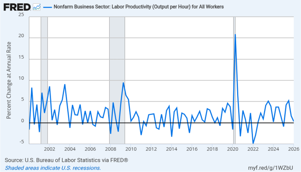
Warsh argues that rising productivity from the spread of AI will allow the Fed to keep the target for the federal funds rate lower without risking rising inflation in a way similar to Greenspan’s policy in the 1990s. The following figure shows productivity growth, as measured by the annual rate of change of output per hour worked for the nonfarm business sector, during the period from the first quarter of 2000 through the first quarter of 2026. Productivity has grown at an annual rate of 2.6 percent since the first quarter of 2023 as opposed to a rate of 2.0 percent for the whole period since 2000.

Productivity moves erratically over short periods, so it’s not yet clear whether AI, in fact, will cause a sustained increase in output per hour worked. Many economists argue that over the short run, AI may be increasing demand more than it is increasing supply. The most important effect of AI to this point might be the surge in demand for data centers, which accounts for more than a third of new capital investment. In addition, Warsh’s remarks at his press conference following the last FOMC meeting made it clear that his top priority is to bring inflation back to the Fed’s 2 percent target. Investors trading in the federal funds futures market now assign a 60 percent probability to the FOMC raising its target for the federal funds rate at its September meeting.

If Warsh intends to follow Greenspan’s strategy of keeping interest rates low to facilitate rapid economic growth during a surge in productivity, he likely won’t begin doing so until well into 2027.

Mokyr, Aghion, and Howitt Win 2025 Nobel Prize in Economics

Joel Mokyr (photo from news.northwestern. edu)

Philippe Aghion (photo from philippeaghion.com)

Peter Howitt (photo from brown.edu)

For most of human history there was little to no economic growth. Until the nineteenth century, the average person everywhere in the world lived at a subsistence level. For example, although the Roman Empire controlled most of Southern and Western Europe, the Near East, and North Africa for more than 400 years, the living standard of the average citizen of the Empire was no higher at the end of the Empire than it had been at the beginning.

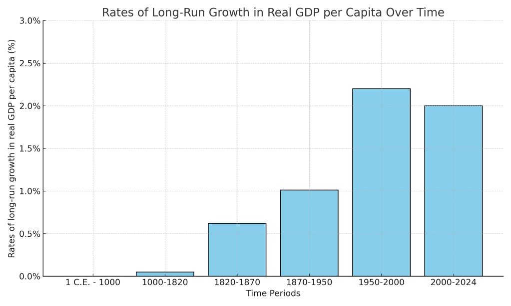
Economists typically measure economic growth by the rate of increase in real GDP per capita. The following figure, updated from Chapter 11 of Macroeconomics (Chapter 21 of Economics), shows the slow pace of growth in real GDP per capita in the world economy from the year 1 to the year 1820 and the much faster rates of growth over the following periods. As discussed in Chapter 11, the figure relies on data compiled by Angus Maddison of University of Groningen in the Netherlands and—for recent years—data from the World Bank.

This year’s three Nobelists have contributed to understanding why economic growth accelerated sharply in the nineteenth century and why England was the first country to experienced sustained increases in real GDP per capita—an event labeled the Industrial Revolution. Joel Mokyr of Northwestern University has conducted decades of research into which innovations were crucial to economic growth and the institutional and economic advantages that allowed entrepreneurs in England to use those innovations to expand production much more rapidly than had happened before. Philippe Aghion of Collège de France and INSEAD and Peter Howitt of Brown University have focused on formally modeling the process of creative destruction that underlies sustained economic growth. The classic discussion of creative destruction appears in Joseph Schumpeter’s book Capitalism, Socialism, and Democracy, published in 1942.

In Macroeconomics Chapter 21, we discuss the process of creative destruction in the context of economic growth. Creative destruction occurs as technological change results in new products that drive firms producing older products out of business. Examples are automobiles driving out of business producers of horse-drawn carriages in the early twentieth century. Or Netflix and other movie streaming sites driving video rental stores out of business in more recent years.

The Nobel Committee’s announcement of the prize can be found here. A longer discussion of the Nobelists’ work can be found here. The scope of their research can be seen by reviewing their curricula vitae, which can be found here, here, and here. The amount of the prize this years is 11 million Swedish kronor (about $1.2 million). Mokyr receives half and Aghion and Howitt receive the other half.

What Will the U.S. Economy Be Like in 50 Years? Glenn Predicts!

Image generated by ChatGPT

A Stronger Safety Net

Modern industrial capitalism’s bounty has been breathtaking globally and especially in the U.S. It’s tempting, then, to look at critics in the crowd in Monty Python’s “Life of Brian” as they ask, “What have the Romans ever do for us?,” only to be confronted with a large list of contributions. But, in fact, over time, American capitalism has been saved by adapting to big economic changes.

We’re at another turning point, and the pattern of American capitalism’s keeping its innovative and disruptive core by responding, if sometimes slowly, to structural shocks will play out as follows. 

The magnitude, scope and speed of technological change surrounding generative artificial intelligence will bring forth a new social insurance aimed at long-term, not just cyclical, impacts of disruption. For individuals, it will include support for work, community colleges and training, and wage insurance for older workers. For places, it will include block grants to communities and areas with high structural unemployment to stimulate new business and job opportunities. Such efforts are a needed departure from a focus on cyclical protection from short-term unemployment toward a longer-term bridge of reconnecting to a changing economy. 

These ideas, like America’s historical big responses in land-grant colleges and the GI Bill, combine federal funding support with local approaches (allowing variation in responses to local business and employment opportunities), another hallmark of past U.S. economic policy. 

With a stronger economic safety net, the current push toward higher tariffs and protectionism will gradually fade. Protectionism is a wall against change, but it is one that insulates us from progress, too. 

A growing budget deficit and strains on public finances will lead to a reliance on consumption taxes to replace the current income tax system; continuing to raise taxes on saving and investment will arrest growth prospects. For instance, a tax on business cash flow, which places a levy on a firm’s revenue minus all expenses including investment, would replace taxes on business income. Domestic production would be enhanced by adding a border adjustment to business taxes—exports would be exempt from taxation, but companies can’t claim a deduction for the cost of imports.

That reform allows a shift from helter-skelter tariffs to tax reform that boosts investment and offers U.S. and foreign firms alike an incentive to invest in the U.S. 

These ideas to retain opportunity amid creative destruction will also refresh American capitalism as the nation celebrates its 250th anniversary. They also celebrate the classical liberal ideas of Adam Smith, whose treatise “The Wealth of Nations” appeared the same year. This refresh marries competition’s role in “The Wealth of Nations” and American capitalism with the ability to compete, again a feature of turning points in capitalism in the U.S.

Decades down the road, this “Project 2026” will have preserved the bounty and mass prosperity of American capitalism.

These observations first appeared in the Wall Street Journal, along with predictions from six other economists and economic historians.

Is it 1987 for AI?

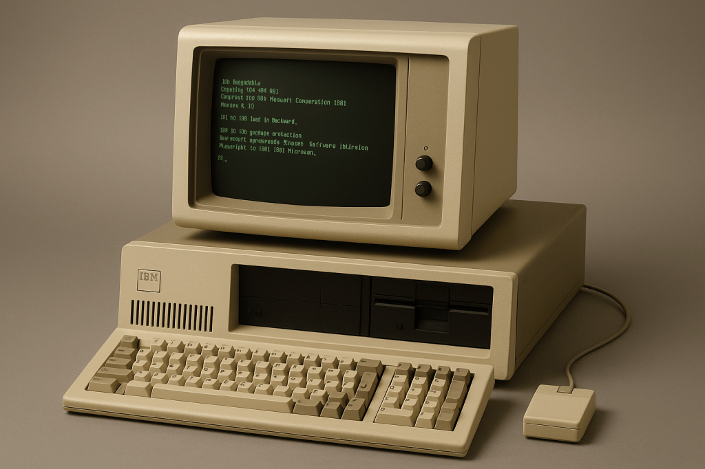
Image generated by ChatGPT 5 of a 1981 IBM personal computer.

The modern era of information technology began in the 1980s with the spread of personal computers. A key development was the introduction of the IBM personal computer in 1981. The Apple II, designed by Steve Jobs and Steve Wozniak and introduced in 1977, was the first widely used personal computer, but the IBM personal computer had several advantages over the Apple II. For decades, IBM had been the dominant firm in information technology worldwide. The IBM System/360, introduced in 1964, was by far the most successful mainframe computer in the world. Many large U.S. firms depended on IBM to meet their needs for processing payroll, general accounting services, managing inventories, and billing.

Because these firms were often reliant on IBM for installing, maintaining, and servicing their computers, they were reluctant to shift to performing key tasks with personal computers like the Apple II. This reluctance was reinforced by the fact that few managers were familiar with Apple or other early personal computer firms like Commodore or Tandy, which sold the TRS-80 through Radio Shack stores. In addition, many firms lacked the technical staffs to install, maintain, and repair personal computers. Initially, it was easier for firms to rely on IBM to perform these tasks, just as they had long been performing the same tasks for firms’ mainframe computers.

By 1983, the IBM PC had overtaken the Apple II as the best-selling personal computer in the United States. In addition, IBM had decided to rely on other firms to supply its computer chips (Intel) and operating system (Microsoft) rather than develop its own proprietary computer chips and operating system. This so-called open architecture made it possible for other firms, such as Dell and Gateway, to produce personal computers that were similar to IBM’s. The result was to give an incentive for firms to produce software that would run on both the IBM PC and the “clones” produced by other firms, rather than produce software for Apple personal computers. Key software such as the spreadsheet program Lotus 1-2-3 and word processing programs, such as WordPerfect, cemented the dominance of the IBM PC and the IBM clones over Apple, which was largely shut out of the market for business computers.

As personal computers began to be widely used in business, there was a general expectation among economists and policymakers that business productivity would increase. Productivity, measured as output per hour of work, had grown at a fairly rapid average annual rate of 2.8 percent between 1948 and 1972. As we discuss in Macroeconomics, Chapter 10 (Economics, Chapter 20 and Essentials of Economics, Chapter 14) rising productivity is the key to an economy achieving a rising standard of living. Unless output per hour worked increases over time, consumption per person will stagnate. An annual growth rate of 2.8 percent will lead to noticeable increases in the standard of living.

Economists and policymakers were concerned when productivity growth slowed beginning in 1973. From 1973 to 198o, productivity grew at an annual rate of only 1.3 percent—less than half the growth rate from 1948 to 1972. Despite the widespread adoption of personal computers by businesses, during the 1980s, the growth rate of productivity increased only to 1.5 percent. In 1987, Nobel laureate Robert Solow of MIT famously remarked: “You can see the computer age everywhere but in the productivity statistics.” Economists labeled Solow’s observation the “productivity paradox.” With hindsight, it’s now clear that it takes time for businesses to adapt to a new technology, such as personal computers. In addition, the development of the internet, increases in the computing power of personal computers, and the introduction of innovative software were necessary before a significant increase in productivity growth rates occurred in the mid-1990s.

Result when ChatGPT 5 is asked to create an image illustrating ChatGPT

The release of ChatGPT in November 2022 is likely to be seen in the future as at least as important an event in the evolution of information technology as the introduction of the IBM PC in August 1981. Just as with personal computers, many people have been predicting that generative AI programs will have a substantial effect on the labor market and on productivity.

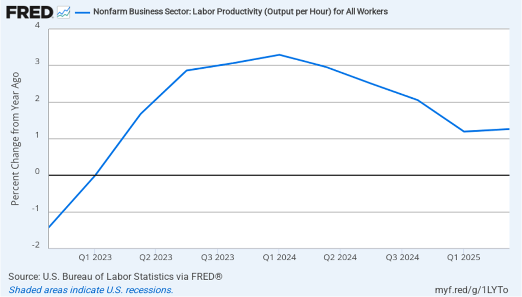
In this recent blog post, we discussed the conflicting evidence as to whether generative AI has been eliminating jobs in some occupations, such as software coding. Has AI had an effect on productivity growth? The following figure shows the rate of productivity growth in each quarter since the fourth quarter of 2022. The figure shows an acceleration in productivity growth beginning in the fourth quarter of 2023. From the fourth quarter of 2023 through the fourth quarter of 2024, productivity grew at an annual rate of 3.1 percent—higher than during the period from 1948 to 1972. Some commentators attributed this surge in productivity to the effects of AI.

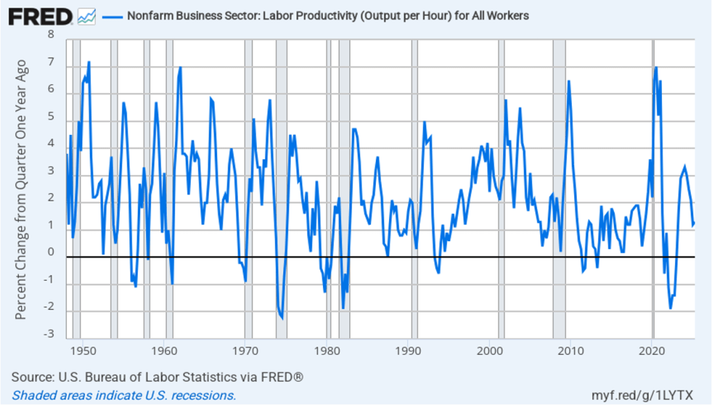
However, the increase in productivity growth wasn’t sustained, with the growth rate in the first half of 2025 being only 1.3 percent. That slowdown makes it more likely that the surge in productivity growth was attributable to the recovery from the 2020 Covid recession or was simply an example of the wide fluctuations that can occur in productivity growth. The following figure, showing the entire period since 1948, illustrates how volatile quarterly rates of productivity growth are.

How large an effect will AI ultimately have on the labor market? If many current jobs are replaced by AI is it likely that the unemployment rate will soar? That’s a prediction that has often been made in the media. For instance, Dario Amodei, the CEO of generative AI firm Anthropic, predicted during an interview on CNN that AI will wipe out half of all entry level jobs in the U.S. and cause the unemployment rate to rise to between 10% and 20%.  

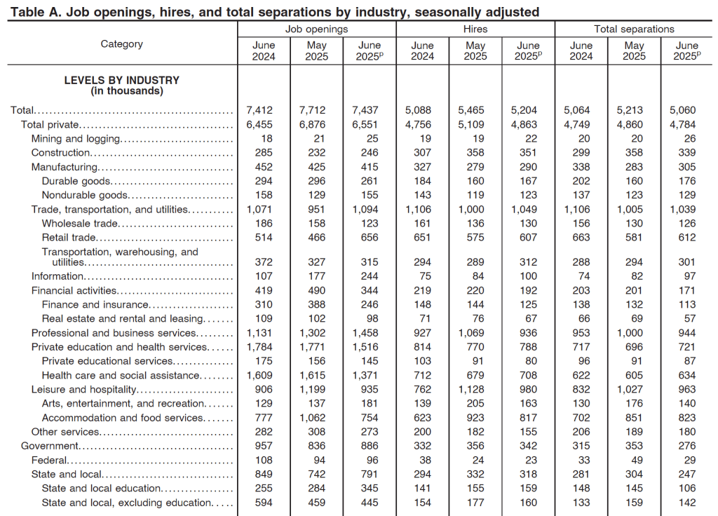
Although Amodei is likely correct that AI will wipe out many existing jobs, it’s unlikely that the result will be a large increase in the unemployment rate. As we discuss in Macroeconomics, Chapter 9 (Economics, Chapter 19 and Essentials of Economics, Chapter 13) the U.S. economy creates and destroys millions of jobs every year. Consider, for instance, the following table from the most recent “Job Openings and Labor Turnover” (JOLTS) report from the Bureau of Labor Statistics (BLS). In June 2025, 5.2 million people were hired and 5.1 million left (were “separated” from) their jobs as a result of quitting, being laid off, or being fired.

Most economists believe that one of the strengths of the U.S. economy is the flexibility of the U.S. labor market. With a few exceptions, “employment at will” holds in every state, which means that a business can lay off or fire a worker without having to provide a cause. Unionization rates are also lower in the United States than in many other countries. U.S. workers have less job security than in many other countries, but—crucially—U.S. firms are more willing to hire workers because they can more easily lay them off or fire them if they need to. (We discuss the greater flexibility of U.S. labor markets in Macroeconomics, Chapter 11 (Economics, Chapter 21).)

The flexibility of the U.S. labor market means that it has shrugged off many waves of technological change. AI will have a substantial effect on the economy and on the mix of jobs available. But will the effect be greater than that of electrification in the late nineteenth century or the effect of the automobile in the early twentieth century or the effect of the internet and personal computing in the 1980s and 1990s? The introduction of automobiles wiped out jobs in the horse-drawn vehicle industry, just as the internet has wiped out jobs in brick-and-mortar retailing. People unemployed by technology find other jobs; sometimes the jobs are better than the ones they had and sometimes the jobs are worse. But economic historians have shown that technological change has never caused a spike in the U.S. unemployment rate. It seems likely—but not certain!—that the same will be true of the effects of the AI revolution. 

Which jobs will AI destroy and which new jobs will it create? Except in a rough sense, the truth is that it is very difficult to tell. Attempts to forecast technological change have a dismal history. To take one of many examples, in 1998, Paul Krugman, later to win the Nobel Prize, cast doubt on the importance of the internet: “By 2005 or so, it will become clear that the Internet’s impact on the economy has been no greater than the fax machine’s.” Krugman, Amodei and other prognosticators of the effects of technological change simply lack the knowledge to make an informed prediction because the required knowledge is spread across millions of people. 

That knowledge only becomes available over time. The actions of consumers and firms interacting in markets mobilize information that is initially known only partially to any one person. In 1945, Friedrich Hayek made this argument in “The Use of Knowledge in Society,” which is one of the most influential economics articles ever written. One of Hayek’s examples is an unexpected decrease in the supply of tin. How will this development affect the economy? We find out only by observing how people adapt to a rising price of tin: “The marvel is that … without an order being issued, without more than perhaps a handful of people knowing the cause, tens of thousands of people whose identity could not be ascertained by months of investigation are made [by the increase in the price of tin] to use the material or its products more sparingly.” People adjust to changing conditions in ways that we lack sufficient information to reliably forecast. (We discuss Hayek’s view of how the market system mobilizes the knowledge of workers, consumers, and firms in Microeconomics, Chapter 2.)

It’s up to millions of engineers, workers, and managers across the economy, often through trial and error, to discover how AI can best reduce the cost of producing goods and services or improve their quality. Competition among firms drives them to make the best use of AI. In the end, AI may result in more people or fewer people being employed in any particular occupation.  At this point, there is no way to know.


New Census Data Highlights the Aging of the U.S. Population

Image generated by ChatGPT 5

In June, the U.S. Census Bureau released its population estimates for 2024. Included was the following graphic showing the change in the U.S. population pyramid from 2004 to 2024. As the graphic shows, people 65 years and older have increased as a fraction of the total population, while children have decreased as a fraction of the total population. (The Census considers everyone 17 and younger to be a child.) Between 2004 and 2024, people 65 and older increased from 12.4 percent of the population to 18.0 percent. People younger than 18 fell from 25.0 percent of the population in 2004 to 21.5 percent in 2024.

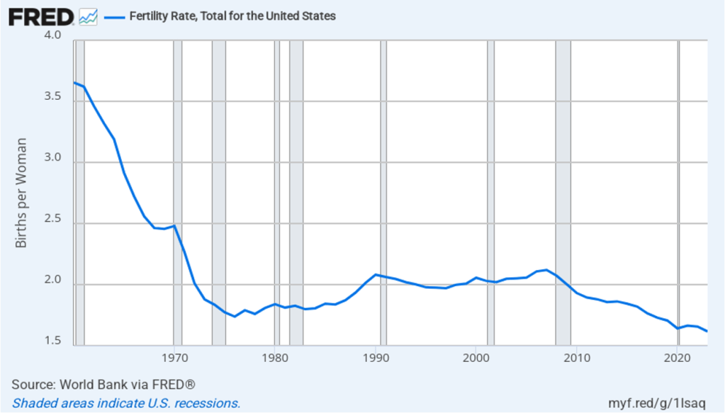
The aging of the U.S. population reflects falling birth rates. Demographers and economists typically measure birth rates as the total fertility rate (TFR), which is defined by the World Bank as: “The number of children that would be born to a woman if she were to live to the end of her childbearing years and bear children in accordance with age-specific fertility rates currently observed.” The TFR has the advantage over the simple birth rate—which is the number of live births per thousand people—because the TFR corrects for the age structure of a country’s female population. Leaving aside the effects of immigration and emigration, a TFR of 2.1 is necessary to keep a country’s population stable. Stated another way, a country needs a TFR of 2.1 to achieve replacement level fertility. A country with a TFR above 2.1 experiences long-run population growth, while a country with a TFR of less than 2.1 experiences long-run population decline.

The following figure shows the TFR for the United States for each year between 1960 and 2023. Since 1971, the TFR has been below 2.1 in every year except for 2006 and 2007. Immigration has helped to offset the effects on population growth of a TFR below 2.1.

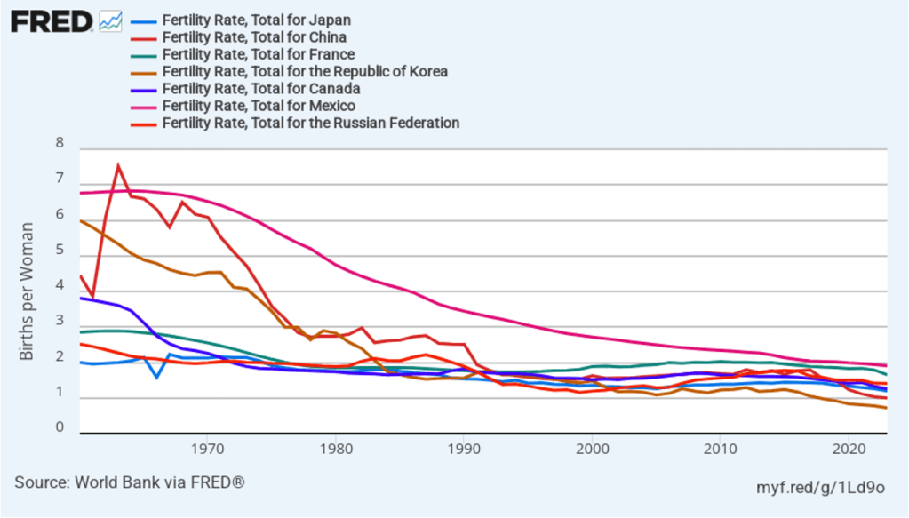
The United States is not alone in experiencing a sharp decline in its TFR since the 1960s. The following figure shows some other countries that currently have below replacement level fertility, including some countries—such as China, Japan, Korea, and Mexico—in  which TFRs were well above 5 in the 1960s. In fact, only a relatively few countries, such as Israel and some countries in sub-Saharan Africa are still experiencing above replacement level fertility.

An aging population raises the number of retired people relative to the number of workers, making it difficult for governments to finance pensions and health care for older people. We discuss this problem with respect to the U.S. Social Security and Medicare programs in an Apply the Concept in Macroeconomics, Chapter 16 (Economics, Chapter 26 and Essentials of Economics, Chapter 18). Countries experiencing a declining population typically also experience lower rates of economic growth than do countries with growing populations. Finally, as we discuss in an Apply the Concept in Microeconomics, Chapter 3, different generations often differ in the mix of products they buy. For instance, a declining number of children results in declining demand for diapers, strollers, and toys.

Glenn on Policies to Increase Economic Growth and Reduce the Federal Budget Deficit

Image generated by ChatGTP 40

Glenn, along with co-authors Douglas Elmendorf of Harvard’s Kennedy School and Zachary Liscow of the Yale Law School, has written a new National Bureau of Economic Research working paper: “Policies to Reduce Federal Budget Deficits by Increasing Economic Growth”

Here’s the abstract:

Could policy changes boost economic growth enough and at a low enough cost to meaningfully reduce federal budget deficits? We assess seven areas of economic policy: immigration of high-skilled workers, housing regulation, safety net programs, regulation of electricity transmission, government support for research and development, tax policy related to business investment, and permitting of infrastructure construction. We find that growth-enhancing policies almost certainly cannot stabilize federal debt on their own, but that such policies can reduce the explicit tax hikes, spending cuts, or both that are needed to stabilize debt. We also find a dearth of research on the likely impacts of potential growth-enhancing policies and on ways to design such policies to restrain federal debt, and we offer suggestions for ways to build a larger base of evidence.

The full working paper can be found at this link.

Glenn Proposes Tax Reforms to Aid Economic Growth

Photo of the Internal Revenue Service building in Washington, DC from the Associated Press via the Wall Street Journal

The following op-ed by Glenn first appeared in the Wall Street Journal.

The GOP Tax Bill Could Solve the Tariff Problem

The economy and financial markets nervously await the July 8 end of the 90-day pause of the Trump administration’s “reciprocal” tariffs. But four days earlier, Republicans can allay those fears with a pro-growth policy that advances President Trump’s Made in America agenda without tariffs. The fix: tax reform.

July 4 is the date that Treasury Secretary Bessent has predicted Congress and the White House will have ready a 2.0 version of the landmark Tax Cut and Jobs Act of 2017, or TCJA. Without congressional action, some of these reforms will expire at the end of 2025, killing changes that still benefit the economy. Corporate tax changes, in particular, boosted investment and growth. These should remain the focal point of this next tax bill—for many reasons. Done right, corporate tax reform could advance President Trump’s goal to bring investment to American production without using economy-roiling tariffs. Call it TCJA+.

Renewing some parts of the original TCJA will help investment in the U.S. The 2017 reform offered incentives for investment in new businesses by allowing them to expense the cost of assets, rather than writing them off over time. But these benefits were set to be phased out from 2023 to 2026, removing a key pro-growth element of the earlier law.

Then there are two new provisions Republicans should add to secure Mr. Trump’s goal to have more made in America. Both were in the original 2016 House Republican tax reform blueprint.

First, Congress should change business taxation from the current income tax to a cash-flow tax, which taxes a firm’s revenue, minus all its expenses, including investment. Long championed by economists and tax-law experts, a cash-flow tax would allow businesses to expense investment immediately. It would also disallow nonfinancial companies from making interest deductions, because unlike an income tax, a cash-flow tax treats debt and equity the same. This removes an important tax incentive for firms to allow themselves to be leveraged. A cash-flow tax is also much simpler than a corporate income tax, which requires complex depreciation schedules. Most important, the reform would stimulate business investment.

Second, legislators should add a border adjustment to corporate taxes. That would deny companies a tax deduction for expenses of inputs imported from abroad, while exempting U.S. exports from taxation. As the Trump administration has observed, other countries already use border adjustments in their value-added taxes on consumption. America uses a similar mechanism in state and local retail taxes, too. If you buy a kitchen appliance in New York, you pay New York sales tax, even if it was made in Ohio. Sales tax applies only where the good is sold, not where it originates.

Though distinct from tariffs, border adjustments can promote domestic production. Adding a border adjustment to the federal corporate tax would eliminate any extra tax businesses suffer now simply as a consequence of producing in the U.S. Though the 2017 law made the U.S. tax system more globally competitive by lowering the corporate income tax rate from 35% to 21%, it’s still higher than in many other countries, which attract production with low cost. A border adjustment would remove this incentive for American firms to locate profits or activities abroad, while increasing incentives for non-U.S. firms to locate activities within our borders.

As with the original pro-investment features in the 2017 law, this TCJA+ reform would increase investment and incomes—and thereby revenue. For the original TCJA, when the Congressional Budget Office included the macroeconomic effects of higher incomes buoyed by the reforms’ pro-growth elements, the CBO reduced the estimated revenue loss from the tax cuts by almost 30%. Changing the corporate income tax to a cash-flow levy would similarly increase revenue by removing taxes on what economists call the “normal return” on investment, or the cost of capital. Companies would instead pay only on profits above this amount. A border adjustment can likewise raise substantial revenue over the next decade because imports (which would receive no deduction) are larger than exports (which would no longer be taxed).

The higher revenue these two TCJA+ provisions promise could be used to lower the tax rate on business cash flow or to fund other tax-policy objectives. Importantly, that revenue can replace revenue raised from the tariffs the Trump administration had planned to implement on July 8. These two tax provisions would accomplish the president’s America-first and revenue objectives without destabilizing businesses with whipsawing tariffs.

Finally, TCJA+ would offer another big benefit: It would move the U.S. toward independence from political meddling in the economy via targeted protection or subsidies. This added predictability and breathing room for investment would be one more reason to produce in America. Pluses indeed.

Glenn on the Importance of Research

An image generated by GTP-4o illustrating research.

This opinion column by Glenn appeared in the Financial Times on March 10.

The Trump administration has wisely emphasised raising America’s rate of economic growth. But growth doesn’t just happen. It is the byproduct of innovation both radical (think of the emergence of generative artificial intelligence) and gradual (such as improvements in manufacturing processes or transport). Many economic factors influence innovation, but research and development is key. While this can be privately or publicly funded, the latter can support basic research with spillovers to many companies and applications.

Therein lies the rub: the new administration’s growth agenda is joined by a significant effort to reduce government spending, spearheaded by the so-called Department of Government Efficiency. Some spending restraint can enhance growth by reducing interest rates or reallocating funds towards more investment-oriented activities. But cuts to R&D, as the administration is advocating at the National Institutes of Health (NIH), National Science Foundation (NSF), Department of Energy (DoE) and NASA, are counter-productive. They will limit innovation and growth.

The link between R&D and productivity growth has a long pedigree in economics and has generally been acknowledged by US policymakers. In the mid-1950s, economist Robert Solow made the Nobel Prize-winning conclusion that sustained output growth is not possible without technological progress. Decades later, former World Bank chief economist Paul Romer added another Nobel Prize-winning insight: growth reflected the intentional adoption of new ideas, so could be affected by research incentives.

It is well known that research is undervalued by private companies. Private funders of R&D don’t capture all its benefits. The social returns of R&D are two to four times higher than private returns. These high returns are enabled in the US by federal funding. For example, publicly funded research at the NIH has been found to significantly impact private development of new drugs.

In a comprehensive study, Andrew Fieldhouse and Karel Mertens classify major changes in non-defence R&D funding by the DoE, Nasa, NIH and NSF over the postwar period. They estimate implied returns of as much as 200 per cent — raising US economic output by $2 per dollar of funding. This is substantially higher than recent estimates of returns to private R&D. According to the Congressional Budget Office, the high returns to public funding are more than 10 times that on public investment in infrastructure. With the higher tax revenue generated from additional GDP, an increase in R&D funding more than pays for itself.

In aggregate, productivity gains from federal R&D funding are substantial. Indeed, Fieldhouse and Mertens estimate that government-funded R&D amounts to about one-fifth of productivity growth (measured as output growth less all input growth) in the US since the second world war.

Combined with the high social returns of government-funded R&D, it is essential that policymakers in the current administration acknowledge the risks of underfunding R&D. Spending cuts are clearly harmful to productivity and even budget outcomes.

A shift towards government-financed R&D does not imply that policy in these areas should be beyond review. Some economists have questioned whether current R&D projects take sufficiently high scientific risks, particularly on the ideas of younger scholars. And policymakers can certainly investigate whether indirect cost subsidies to universities and laboratories—in addition to the direct costs of research—are set at the appropriate levels. But, if growth is the objective, the presumption must be that additional public spending on R&D is worthwhile.

Federal support for growth-oriented R&D can extend beyond research grants. Publicly supported applied research centres around the country offer a mechanism to collaborate with local universities and business networks to disseminate ideas to practice. This builds upon the agricultural and manufacturing extension services instituted by 19th-century land-grant colleges that enhanced productivity.

The Trump administration is right to promote growth as a public objective. Spending restraint and fiscal discipline can be growth-enhancing. But all spending is equal. Government-funded R&D is vitally important for innovation and productivity growth. The case is clear.