
What happens when the Fed chair’s seat is about to change hands—and inflation still won’t behave? In this episode of the Hubbard & O’Brien Economics Podcast, Tony O’Brien and Glenn Hubbard break down the looming transition from Jerome Powell to Kevin Warsh, what the latest inflation and energy-price pressures mean for interest rates, and why navigating the FOMC could be Warsh’s toughest test yet. They also unpack the Fed’s massive balance sheet, the regulatory constraints around shrinking it, and a surprising new risk on the horizon: AI-driven security threats that could expose vulnerabilities across the financial system. If you want a clear, candid take on where monetary policy may be headed next, this is the listen.
Category: Ch20: Economic Growth, the Financial System, and Business Cycles
2-28-26 Podcast – Glenn Hubbard & Tony O’Brien revisit Tariffs and AI!
Join authors Glenn Hubbard and Tony O’Brien as they discuss how core economic principles illuminate two of the most pressing policy debates facing the economy today: tariffs and artificial intelligence. Drawing on a recent Supreme Court decision striking down broad tariff increases, Hubbard and O’Brien explain why economists view tariffs as taxes, who ultimately bears their burden, and how trade policy uncertainty shapes business decisions, inflation, and economic growth—bringing textbook concepts like tax incidence, intermediate goods, and GDP measurement vividly to life. The conversation then turns to AI, where they cut through market hype and dire predictions to place generative AI in historical context as a general‑purpose technology, comparing it to past innovations that transformed jobs without eliminating work. Along the way, they explore how AI can both substitute for and complement labor, why fears of mass unemployment are likely overstated, and what economists can—and cannot yet—say about AI’s long‑run effects on productivity, profits, and the labor market.
New Real GDP Data Shows that Growth Slowed Substantially in the Fourth Quarter … or Did It?

Image created by ChatGPT
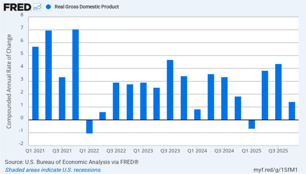
Recent macro data had been showing relatively strong growth in output and steady growth in employment. This morning’s release of the initial estimate of real GDP growth for the fourth quarter of 2025 from the Bureau of Economic Analysis (BEA) was expected to show continuing solid growth. (The report can be found here.) Instead, the BEA estimates that real GDP increased in the fourth quarter by only 1.4 percent measured at an annual rate. Growth was down sharply from the 4.4 percent increase in the third quarter of 2025. Economists surveyed by the Wall Street Journal had forecast a 2.5 percent increase. The following figure shows the estimated rates of GDP growth in each quarter beginning with the first quarter of 2021.
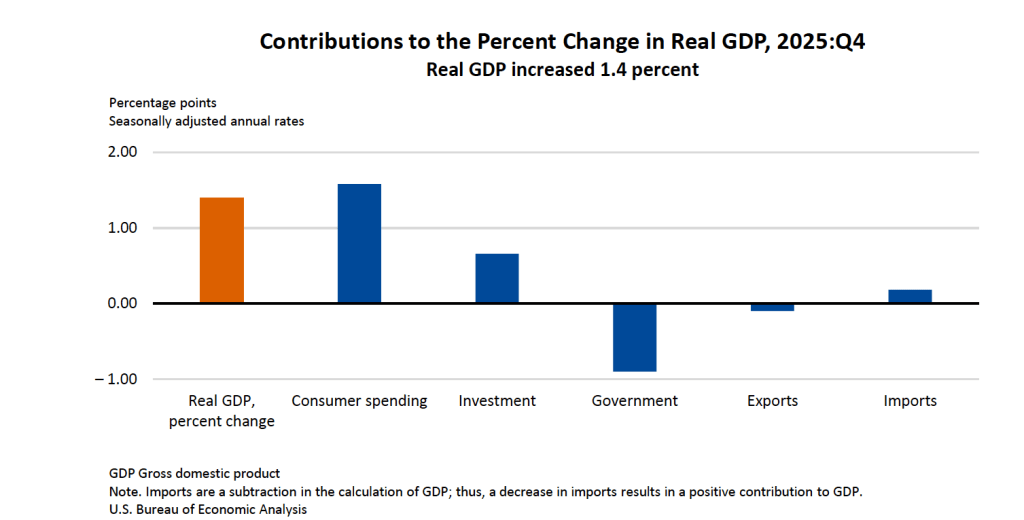
As the following figure—taken from the BEA report—shows, the decline in real government expenditures of –0.90 percent at an annual rate was the most important factor contributing to the slowing growth in real GDP during the fourth quarter. The decline in government expenditures is largely attributable to the federal government shutdown, which lasted from October 1, 2025 to November 12, 2025.
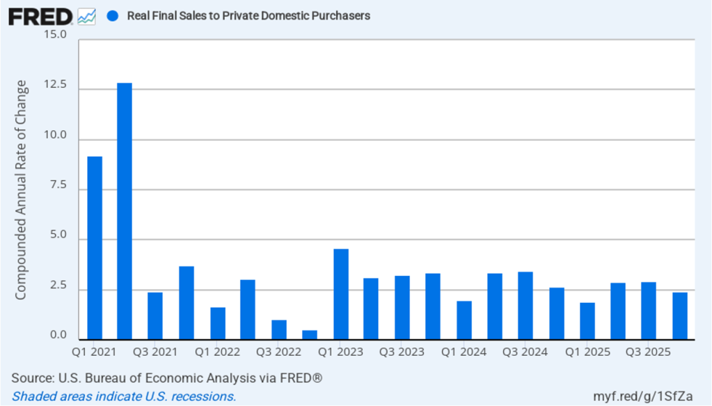
As we’ve discussed in previous blog posts, to better gauge the state of the economy, policymakers—including Fed Chair Jerome Powell—often prefer to strip out the effects of imports, inventory investment, and government expenditures—which can be volatile—by looking at real final sales to private domestic purchasers, which includes only spending by U.S. households and firms on domestic production. As the following figure shows, real final sales to domestic purchasers increased by 2.4 percent at an annual rate in the fourth quarter, which was well above the 1.4 percent increase in real GDP and also above the U.S. economy’s expected long-run annual real growth rate of 1.8 percent. Note also that real final sales to private domestic purchasers grew by 2.9 percent in the third quarter, during which real GDP grew by 4.4 percent, and by 1.9 percent in the first quarter of 2025, when real GDP declined by 0.6 percent. So this measure of output is more stable and likely is a better indicator of the underlying growth rate in the economy than is growth in real GDP.
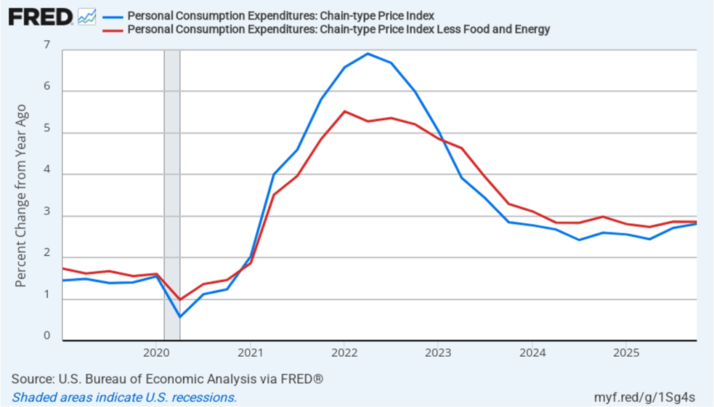
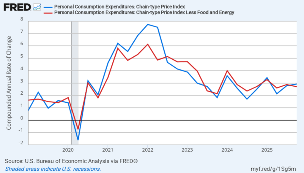
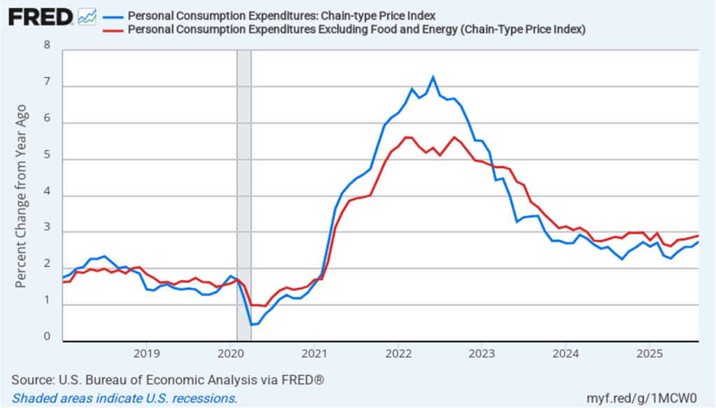
The BEA report this morning also included quarterly data on the personal consumption expenditures (PCE) price index. The Fed relies on annual changes in the PCE price index to evaluate whether it’s meeting its 2 percent annual inflation target. The following figure shows headline PCE inflation (the blue line) and core PCE inflation (the red line)—which excludes energy and food prices—for the period since the first quarter of 2019, with inflation measured as the percentage change in the PCE from the same quarter in the previous year. In the fourth quarter of 2025, headline PCE inflation was 2.8 percent, up slightly from 2.7 percent in the third quarter. Core PCE inflation in the third quarter was 2.9 percent, unchanged from the third quarter. Both headline PCE inflation and core PCE inflation remained above the Fed’s 2 percent annual inflation target.
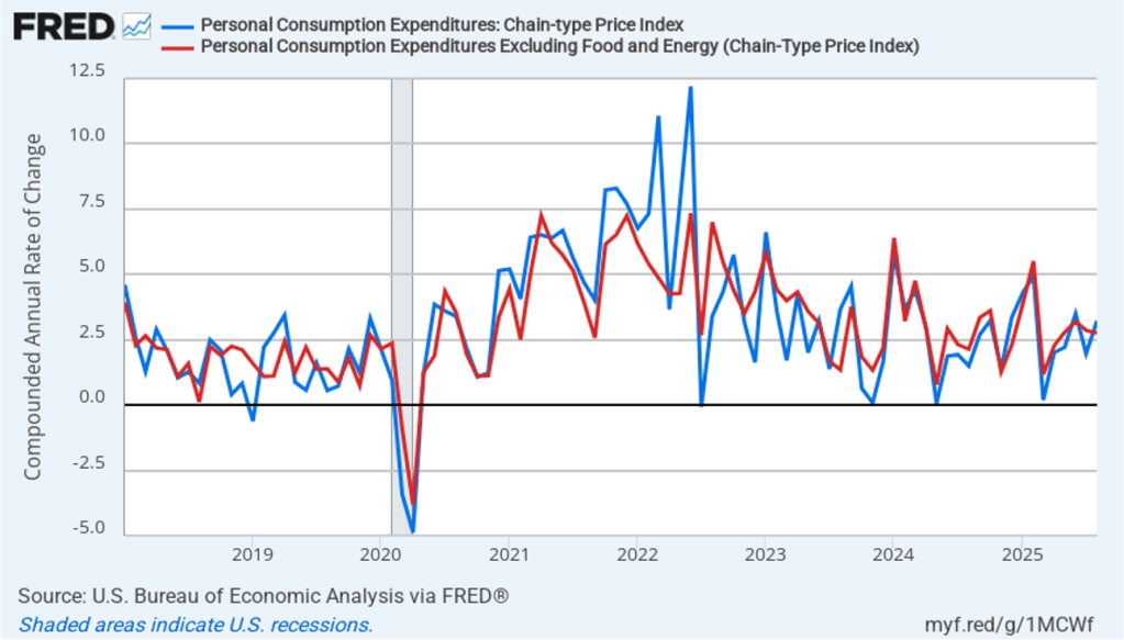
The following figure shows quarterly PCE inflation and quarterly core PCE inflation calculated by compounding the current quarter’s rate over an entire year. Measured this way, headline PCE inflation increased to 2.9 percent in the fourth quarter of 2025, up from to 2.8 percent in the third quarter. Core PCE inflation fell to 2.7 percent in the fourth quarter of 2025 from 2.9 percent in the third quarter. Measured this way, both core and headline PCE inflation were also above the Fed’s target.
Today was also notable for a decision from the U.S. Supreme Court that invalidated some of the Trump administration’s tariff increases that began to be implemented in April 2025. President Trump announced this afternoon that he would impose a new 10 percent across-the-board tariff, relying on Section 122 of the Trade Act of 1974, rather than on the International Emergency Economic Powers Act (IEEPA), which the Supreme Court ruled today did not authorize presidents to unilaterally impose tariffs.
Today’s developments appeared unlikely to have much effect on the views of the members of the Fed’s policymaking Federal Open Market Committee (FOMC). The FOMC is unlikely to lower its target for the federal funds rate at its next meeting on March 17–18. The probability that investors in the federal funds futures market assign to the FOMC keeping its target rate unchanged at that meeting increased only slightly from 94.6 percent yesterday to 96.0 percent this afternoon.
11-07-25- Podcast – Authors Glenn Hubbard & Tony O’Brien discuss Tariffs, AI, and the Economy
Glenn Hubbard and Tony O’Brien begin by examining the challenges facing the Federal Reserve due to incomplete economic data, a result of federal agency shutdowns. Despite limited information, they note that growth remains steady but inflation is above target, creating a conundrum for policymakers. The discussion turns to the upcoming appointment of a new Fed chair and the broader questions of central bank independence and the evolving role of monetary policy. They also address the uncertainty surrounding AI-driven layoffs, referencing contrasting academic views on whether artificial intelligence will complement existing jobs or lead to significant displacement. Both agree that the full impact of AI on productivity and employment will take time to materialize, drawing parallels to the slow adoption of the internet in the 1990s.
The podcast further explores the recent volatility in stock prices of AI-related firms, comparing the current environment to the dot-com bubble and questioning the sustainability of high valuations. Hubbard and O’Brien discuss the effects of tariffs, noting that price increases have been less dramatic than expected due to factors like inventory buffers and contractual delays. They highlight the tension between tariffs as tools for protection and revenue, and the broader implications for manufacturing, agriculture, and consumer prices. The episode concludes with reflections on the importance of ongoing observation and analysis as these economic trends evolve.
Pearson Economics · Hubbard OBrien Economics Podcast – 11-06-25 – Economy, AI, & Tariffs
Older People Have Become Relatively Wealthier While Younger People Have Become Relatively Less Wealthy

Image created by ChatGPT
There has been an ongoing debate about whether Millennials and people in Generation Z are better off or worse off economically than are Baby Boomers. Edward Wolff of New York University recently published a National Bureau of Economic Research (NBER) working paper that focuses on one aspect of this debate—how the wealth of households headed by someone 75 years and older changed relative to the wealth of households headed by someone 35 years and younger during the period from 1983 to 2022.
Wolff uses data from the Federal Reserve’s Survey of Consumer Finances to measure the wealth, or net worth, of people in these age groups—the market value of their financial assets minus the market value of their financial liabilities. He includes in his measure of assets the market value of people’s real estate holdings—including their homes—stocks and bonds, bank deposits, contributions to defined contribution pension funds, unincorporated businesses, and trust funds. He includes in his measure of liabilities people’s mortgage debt, consumer debt—including credit card balances—and other debt, such as educational loans. Because Wolff wants to focus on that part of wealth that is available to be spent on consumption, he refers to it as financial resources, and he excludes from his wealth measure the present value of future Social Security payments and the present value of future defined contribution pension benefits.
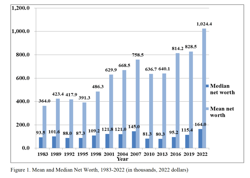
The following figure from Wolff’s paper shows that, using his definition, both median and mean wealth have increased substantially from 1987 to 2o22. Note that both measures of average wealth declined during the Great Recession and Global Financial Crisis of 2007–2009. Median wealth declined by nearly 44 percent between 2007 and 2010. That median wealth grew much faster than mean wealth over the whole period indicates that wealth inequality.
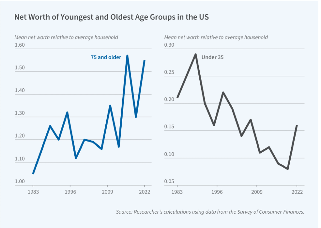
Although the average wealth of all age groups increased over this period, the relative wealth of households 75 years and older rose and the relative wealth of households 35 years and younger fell. The following figure from the NBER Digest illustrates this shift. The 75 and over age group increased its mean net worth from 5 percent greater than the mean net worth of the average household in 1983 to 55 percent of the mean net worth of the average household in 2022. In contrast, the 35 and under age group saw its mean new worth relative to the average household fall from 21 percent in 1983 to 16 percent in 2022. Note, though, that there is significant volatility over time in the relative wealth shares of the two age groups.
What explains the relative increase in wealth among households 75 and over and the relative decrease in wealth among households 35 and under? Wolff identifies three key factors:
“[T]he homeownership rate, total stocks directly and indirectly owned, and home mortgage debt. The homeownership rate is the same in the two years for the youngest group but falls relative to the overall rate, whereas it shoots up for the oldest group both in actual level and relative to the overall average. The value of stock holdings rises for both age groups but vastly more for the oldest households compared to the youngest ones and accounts for a substantial portion of the elderly’s relative wealth gains. Mortgage debt rises in dollar terms for both groups but considerably more in relative terms for the youngest group.”
Perhaps surprisingly, Wolff finds that “despite dire press reports, educational loans fail to appear as a significant factor” in explaining the decline in the relative wealth of younger households.
Mokyr, Aghion, and Howitt Win 2025 Nobel Prize in Economics

Joel Mokyr (photo from news.northwestern. edu)

Philippe Aghion (photo from philippeaghion.com)

Peter Howitt (photo from brown.edu)
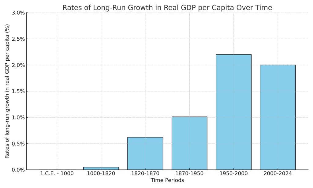
For most of human history there was little to no economic growth. Until the nineteenth century, the average person everywhere in the world lived at a subsistence level. For example, although the Roman Empire controlled most of Southern and Western Europe, the Near East, and North Africa for more than 400 years, the living standard of the average citizen of the Empire was no higher at the end of the Empire than it had been at the beginning.
Economists typically measure economic growth by the rate of increase in real GDP per capita. The following figure, updated from Chapter 11 of Macroeconomics (Chapter 21 of Economics), shows the slow pace of growth in real GDP per capita in the world economy from the year 1 to the year 1820 and the much faster rates of growth over the following periods. As discussed in Chapter 11, the figure relies on data compiled by Angus Maddison of University of Groningen in the Netherlands and—for recent years—data from the World Bank.
This year’s three Nobelists have contributed to understanding why economic growth accelerated sharply in the nineteenth century and why England was the first country to experienced sustained increases in real GDP per capita—an event labeled the Industrial Revolution. Joel Mokyr of Northwestern University has conducted decades of research into which innovations were crucial to economic growth and the institutional and economic advantages that allowed entrepreneurs in England to use those innovations to expand production much more rapidly than had happened before. Philippe Aghion of Collège de France and INSEAD and Peter Howitt of Brown University have focused on formally modeling the process of creative destruction that underlies sustained economic growth. The classic discussion of creative destruction appears in Joseph Schumpeter’s book Capitalism, Socialism, and Democracy, published in 1942.
In Macroeconomics Chapter 21, we discuss the process of creative destruction in the context of economic growth. Creative destruction occurs as technological change results in new products that drive firms producing older products out of business. Examples are automobiles driving out of business producers of horse-drawn carriages in the early twentieth century. Or Netflix and other movie streaming sites driving video rental stores out of business in more recent years.
The Nobel Committee’s announcement of the prize can be found here. A longer discussion of the Nobelists’ work can be found here. The scope of their research can be seen by reviewing their curricula vitae, which can be found here, here, and here. The amount of the prize this years is 11 million Swedish kronor (about $1.2 million). Mokyr receives half and Aghion and Howitt receive the other half.
What Will the U.S. Economy Be Like in 50 Years? Glenn Predicts!
Image generated by ChatGPT
A Stronger Safety Net
Modern industrial capitalism’s bounty has been breathtaking globally and especially in the U.S. It’s tempting, then, to look at critics in the crowd in Monty Python’s “Life of Brian” as they ask, “What have the Romans ever do for us?,” only to be confronted with a large list of contributions. But, in fact, over time, American capitalism has been saved by adapting to big economic changes.
We’re at another turning point, and the pattern of American capitalism’s keeping its innovative and disruptive core by responding, if sometimes slowly, to structural shocks will play out as follows.
The magnitude, scope and speed of technological change surrounding generative artificial intelligence will bring forth a new social insurance aimed at long-term, not just cyclical, impacts of disruption. For individuals, it will include support for work, community colleges and training, and wage insurance for older workers. For places, it will include block grants to communities and areas with high structural unemployment to stimulate new business and job opportunities. Such efforts are a needed departure from a focus on cyclical protection from short-term unemployment toward a longer-term bridge of reconnecting to a changing economy.
These ideas, like America’s historical big responses in land-grant colleges and the GI Bill, combine federal funding support with local approaches (allowing variation in responses to local business and employment opportunities), another hallmark of past U.S. economic policy.
With a stronger economic safety net, the current push toward higher tariffs and protectionism will gradually fade. Protectionism is a wall against change, but it is one that insulates us from progress, too.
A growing budget deficit and strains on public finances will lead to a reliance on consumption taxes to replace the current income tax system; continuing to raise taxes on saving and investment will arrest growth prospects. For instance, a tax on business cash flow, which places a levy on a firm’s revenue minus all expenses including investment, would replace taxes on business income. Domestic production would be enhanced by adding a border adjustment to business taxes—exports would be exempt from taxation, but companies can’t claim a deduction for the cost of imports.
That reform allows a shift from helter-skelter tariffs to tax reform that boosts investment and offers U.S. and foreign firms alike an incentive to invest in the U.S.
These ideas to retain opportunity amid creative destruction will also refresh American capitalism as the nation celebrates its 250th anniversary. They also celebrate the classical liberal ideas of Adam Smith, whose treatise “The Wealth of Nations” appeared the same year. This refresh marries competition’s role in “The Wealth of Nations” and American capitalism with the ability to compete, again a feature of turning points in capitalism in the U.S.
Decades down the road, this “Project 2026” will have preserved the bounty and mass prosperity of American capitalism.
These observations first appeared in the Wall Street Journal, along with predictions from six other economists and economic historians.
Real GDP Growth Revised Up and PCE Inflation Running Slightly Below Expectations
Image generated by ChatGPT
Today (September 26), the Bureau of Economic Analysis (BEA) released monthly data on the personal consumption expenditures (PCE) price index as part of its “Personal Income and Outlays” report. Yesterday, the BEA released its revised estimate of real GDP growth in the second quarter. Taken together, the two reports show that economic growth remains realtively strong and that inflation continues to run above the Fed’s 2 percent annual target.
Taking the inflation report first, the following figure shows headline PCE inflation (the blue line) and core PCE inflation (the red line)—which excludes energy and food prices—for the period since January 2018, with inflation measured as the percentage change in the PCE from the same month in the previous year. In August, headline PCE inflation was 2.7 percent, up from 2.6 percent in July. Core PCE inflation in August was 2.9 percent, unchanged from July. Headline PCE inflation was equal to the forecast of economists surveyed, while core PCE inflation was slightly lower than forecast.
The following figure shows headline PCE inflation and core PCE inflation calculated by compounding the current month’s rate over an entire year. (The figure above shows what is sometimes called 12-month inflation, while this figure shows 1-month inflation.) Measured this way, headline PCE inflation increased from 2.0 percent in July to 3.2 percent in August. Core PCE inflation declined slightly from 2.9 percent in July to 2.8 percent in August. So, both 1-month and 12-month PCE inflation are telling the same story of inflation being well above the Fed’s target. The usual caution applies that 1-month inflation figures are volatile (as can be seen in the figure). In addition, these data likely reflect higher prices resulting from the tariff increases the Trump administration has implemented. Once the one-time price increases from tariffs have worked through the economy, inflation may decline. It’s not clear, however, how long that may take and President Trump indicated yesterday that he may impose new tariffs on pharmaceuticals, large trucks, and furniture.
Fed Chair Jerome Powell has frequently mentioned that inflation in non-market services can skew PCE inflation. Non-market services are services whose prices the BEA imputes rather than measures directly. For instance, the BEA assumes that prices of financial services—such as brokerage fees—vary with the prices of financial assets. So that if stock prices fall, the prices of financial services included in the PCE price index also fall. Powell has argued that these imputed prices “don’t really tell us much about … tightness in the economy. They don’t really reflect that.” The following figure shows 12-month headline inflation (the blue line) and 12-month core inflation (the red line) for market-based PCE. (The BEA explains the market-based PCE measure here.)
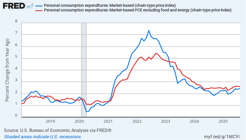
Headline market-based PCE inflation was 2.4 percent in August, unchanged from July. Core market-based PCE inflation was 2.6 percent in August, also unchanged from July. So, both market-based measures show inflation as stable but above the Fed’s 2 percent target.
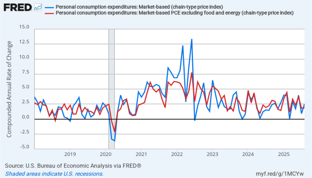
In the following figure, we look at 1-month inflation using these measures. One-month headline market-based inflation increase sharply to 2.5 percent in August from 0.9 percent in July. One-month core market-based inflation increased slightly to 1.9 percent in August from 1.8 percent in July. As the figure shows, the 1-month inflation rates are more volatile than the 12-month rates, which is why the Fed relies on the 12-month rates when gauging how close it is coming to hitting its target inflation rate.
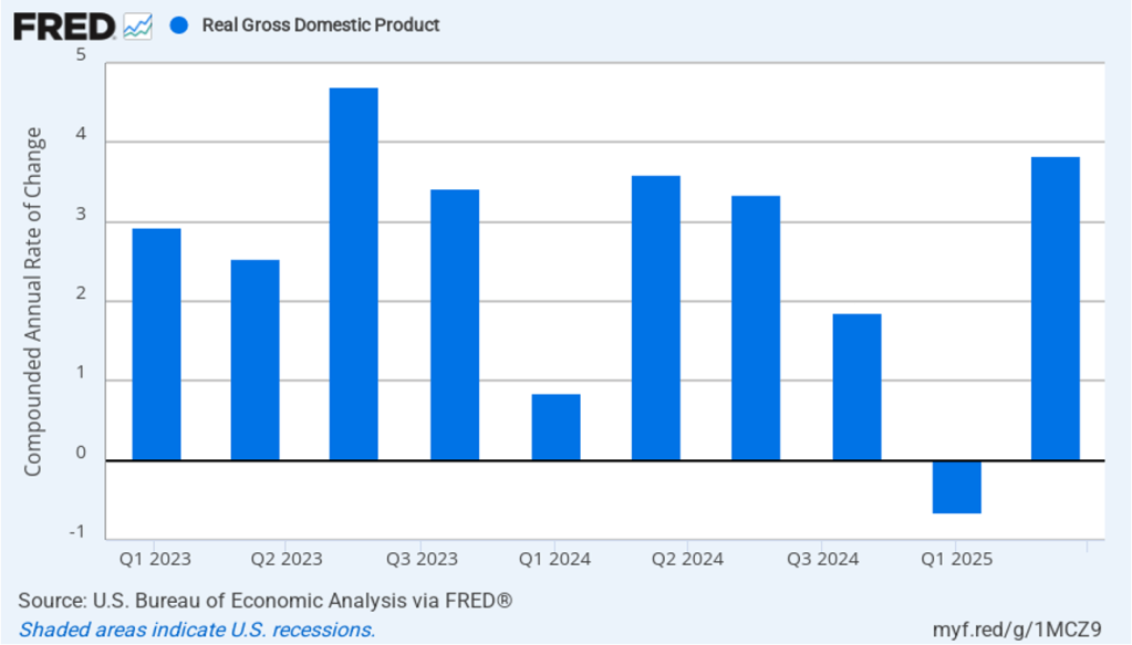
Inflation running above the Fed’s 2 percent target is consistent with relatively strong growth in real GDP. The following figure shows compound annual rates of growth of real GDP, for each quarter since the first quarter of 2023. The value for the second quarter of 2025 is the BEA’s third estimate. This revised estimate increased the growth rate of real GDP to 3.8 percent from the second estimate of 3.3 percent.
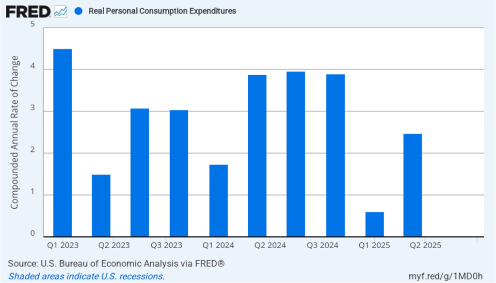
The most important contributor to real GDP growth was growth in real personal consumption expenditures, which, as shown in the following figure, increased aat compound annual rate of 2.5 percent in the second quarter, up from 0.6 percent in the first quarter.
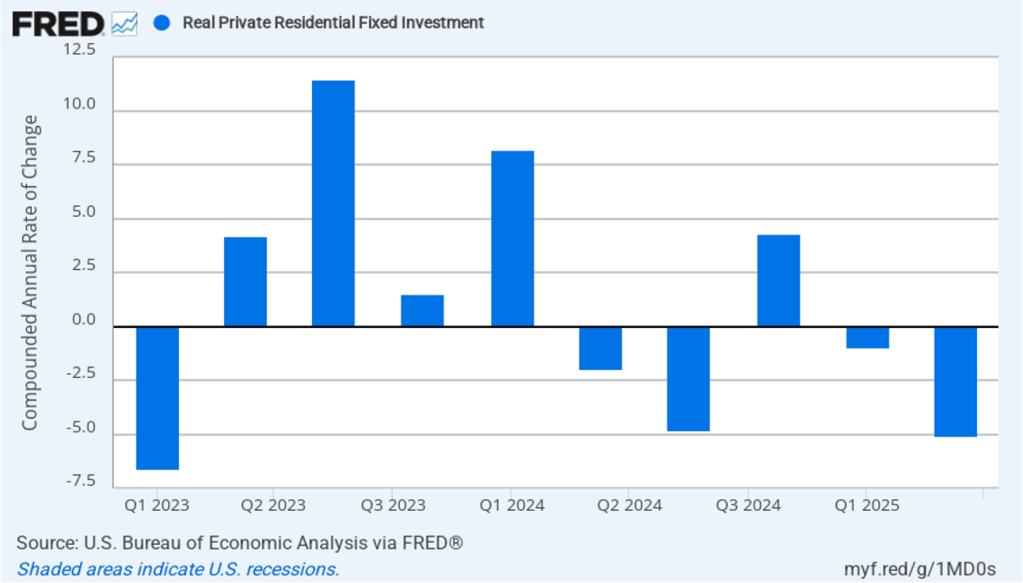
High interest rates continue to hold back residential construction, which declined by a compound annual rate of 5.1 percent in the second quarter after declining 1.0 percent in the first quarter.
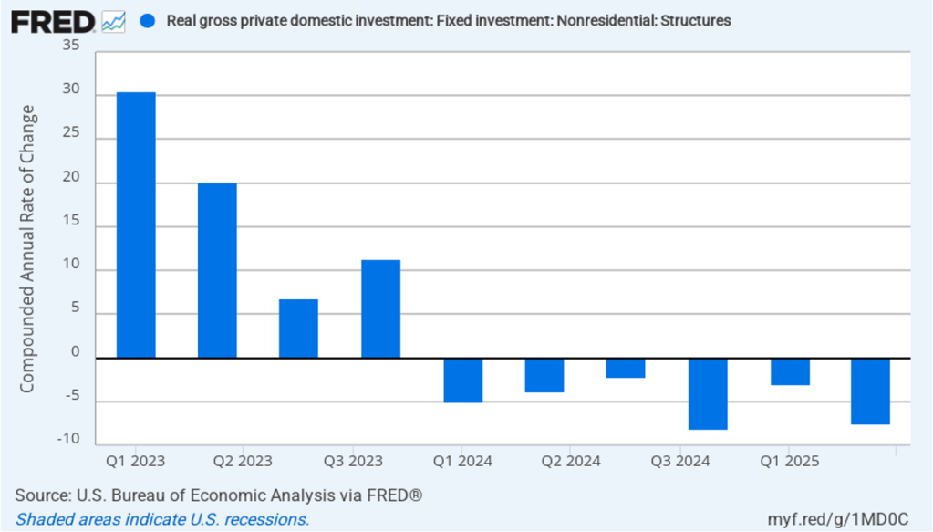
Business investment in structures, such as factories and office buildings, continued a decline that began in the first quarter of 2024.
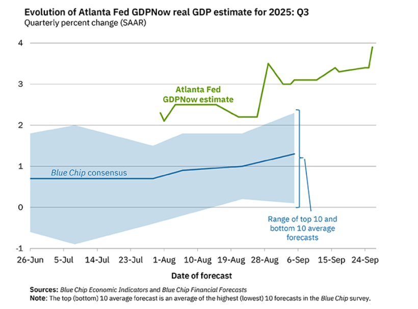
Will the relatively strong growth in real GDP in the second quarter continue in the third quarter? Economists at the Federal Reserve Bank of Atlanta prepare nowcasts of real GDP. A nowcast is a forecast that incorporates all the information available on a certain date about the components of spending that are included in GDP. The Atlanta Fed calls its nowcast GDPNow. As the following figure from the Atlanta Fed website shows, today the GDPNow forecast is for real GDP to grow at an annual rate of 3.9 percent in the third quarter.
Finally, the macroeconomic data released in the last two days has had realtively little effect on the expectations of investors trading federal funds rate futures. Investors assign an 89.8 percent probability to the Federal Open Market Committee (FOMC) cutting its target for the federal funds rate at its meeting on October 28–29 by 0.25 percentage point (25 basis points) from its current range of 4.00 percent to 4.25 percent. That probability is only slightly lower than 91.9 percent probaiblity that investors had assigned to a 25 basis point cut a week ago. However, the probability of the committee cutting its target rate by another 25 basis points at its December 9–10 fell to 67.0 percent today from 78.6 percent one week ago.
Is it 1987 for AI?

Image generated by ChatGPT 5 of a 1981 IBM personal computer.
The modern era of information technology began in the 1980s with the spread of personal computers. A key development was the introduction of the IBM personal computer in 1981. The Apple II, designed by Steve Jobs and Steve Wozniak and introduced in 1977, was the first widely used personal computer, but the IBM personal computer had several advantages over the Apple II. For decades, IBM had been the dominant firm in information technology worldwide. The IBM System/360, introduced in 1964, was by far the most successful mainframe computer in the world. Many large U.S. firms depended on IBM to meet their needs for processing payroll, general accounting services, managing inventories, and billing.
Because these firms were often reliant on IBM for installing, maintaining, and servicing their computers, they were reluctant to shift to performing key tasks with personal computers like the Apple II. This reluctance was reinforced by the fact that few managers were familiar with Apple or other early personal computer firms like Commodore or Tandy, which sold the TRS-80 through Radio Shack stores. In addition, many firms lacked the technical staffs to install, maintain, and repair personal computers. Initially, it was easier for firms to rely on IBM to perform these tasks, just as they had long been performing the same tasks for firms’ mainframe computers.
By 1983, the IBM PC had overtaken the Apple II as the best-selling personal computer in the United States. In addition, IBM had decided to rely on other firms to supply its computer chips (Intel) and operating system (Microsoft) rather than develop its own proprietary computer chips and operating system. This so-called open architecture made it possible for other firms, such as Dell and Gateway, to produce personal computers that were similar to IBM’s. The result was to give an incentive for firms to produce software that would run on both the IBM PC and the “clones” produced by other firms, rather than produce software for Apple personal computers. Key software such as the spreadsheet program Lotus 1-2-3 and word processing programs, such as WordPerfect, cemented the dominance of the IBM PC and the IBM clones over Apple, which was largely shut out of the market for business computers.
As personal computers began to be widely used in business, there was a general expectation among economists and policymakers that business productivity would increase. Productivity, measured as output per hour of work, had grown at a fairly rapid average annual rate of 2.8 percent between 1948 and 1972. As we discuss in Macroeconomics, Chapter 10 (Economics, Chapter 20 and Essentials of Economics, Chapter 14) rising productivity is the key to an economy achieving a rising standard of living. Unless output per hour worked increases over time, consumption per person will stagnate. An annual growth rate of 2.8 percent will lead to noticeable increases in the standard of living.
Economists and policymakers were concerned when productivity growth slowed beginning in 1973. From 1973 to 198o, productivity grew at an annual rate of only 1.3 percent—less than half the growth rate from 1948 to 1972. Despite the widespread adoption of personal computers by businesses, during the 1980s, the growth rate of productivity increased only to 1.5 percent. In 1987, Nobel laureate Robert Solow of MIT famously remarked: “You can see the computer age everywhere but in the productivity statistics.” Economists labeled Solow’s observation the “productivity paradox.” With hindsight, it’s now clear that it takes time for businesses to adapt to a new technology, such as personal computers. In addition, the development of the internet, increases in the computing power of personal computers, and the introduction of innovative software were necessary before a significant increase in productivity growth rates occurred in the mid-1990s.

Result when ChatGPT 5 is asked to create an image illustrating ChatGPT
The release of ChatGPT in November 2022 is likely to be seen in the future as at least as important an event in the evolution of information technology as the introduction of the IBM PC in August 1981. Just as with personal computers, many people have been predicting that generative AI programs will have a substantial effect on the labor market and on productivity.
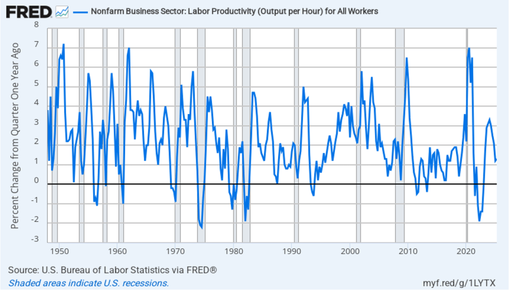
In this recent blog post, we discussed the conflicting evidence as to whether generative AI has been eliminating jobs in some occupations, such as software coding. Has AI had an effect on productivity growth? The following figure shows the rate of productivity growth in each quarter since the fourth quarter of 2022. The figure shows an acceleration in productivity growth beginning in the fourth quarter of 2023. From the fourth quarter of 2023 through the fourth quarter of 2024, productivity grew at an annual rate of 3.1 percent—higher than during the period from 1948 to 1972. Some commentators attributed this surge in productivity to the effects of AI.
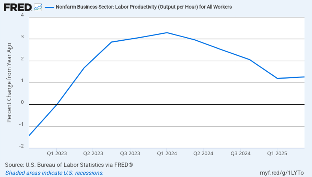
However, the increase in productivity growth wasn’t sustained, with the growth rate in the first half of 2025 being only 1.3 percent. That slowdown makes it more likely that the surge in productivity growth was attributable to the recovery from the 2020 Covid recession or was simply an example of the wide fluctuations that can occur in productivity growth. The following figure, showing the entire period since 1948, illustrates how volatile quarterly rates of productivity growth are.
How large an effect will AI ultimately have on the labor market? If many current jobs are replaced by AI is it likely that the unemployment rate will soar? That’s a prediction that has often been made in the media. For instance, Dario Amodei, the CEO of generative AI firm Anthropic, predicted during an interview on CNN that AI will wipe out half of all entry level jobs in the U.S. and cause the unemployment rate to rise to between 10% and 20%.
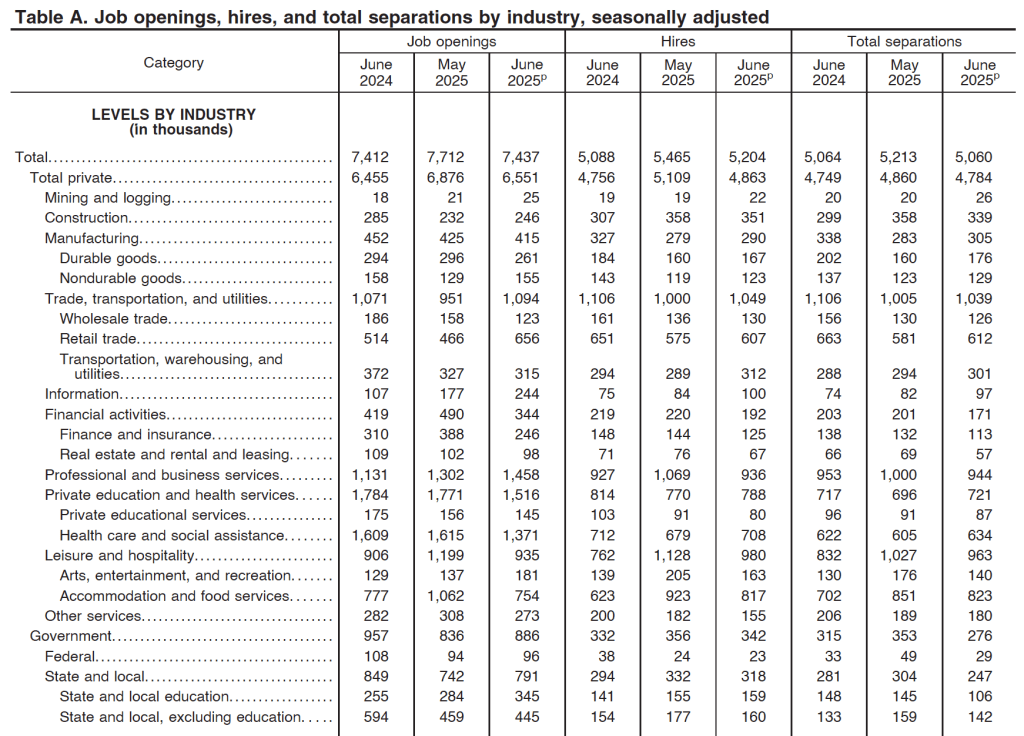
Although Amodei is likely correct that AI will wipe out many existing jobs, it’s unlikely that the result will be a large increase in the unemployment rate. As we discuss in Macroeconomics, Chapter 9 (Economics, Chapter 19 and Essentials of Economics, Chapter 13) the U.S. economy creates and destroys millions of jobs every year. Consider, for instance, the following table from the most recent “Job Openings and Labor Turnover” (JOLTS) report from the Bureau of Labor Statistics (BLS). In June 2025, 5.2 million people were hired and 5.1 million left (were “separated” from) their jobs as a result of quitting, being laid off, or being fired.
Most economists believe that one of the strengths of the U.S. economy is the flexibility of the U.S. labor market. With a few exceptions, “employment at will” holds in every state, which means that a business can lay off or fire a worker without having to provide a cause. Unionization rates are also lower in the United States than in many other countries. U.S. workers have less job security than in many other countries, but—crucially—U.S. firms are more willing to hire workers because they can more easily lay them off or fire them if they need to. (We discuss the greater flexibility of U.S. labor markets in Macroeconomics, Chapter 11 (Economics, Chapter 21).)
The flexibility of the U.S. labor market means that it has shrugged off many waves of technological change. AI will have a substantial effect on the economy and on the mix of jobs available. But will the effect be greater than that of electrification in the late nineteenth century or the effect of the automobile in the early twentieth century or the effect of the internet and personal computing in the 1980s and 1990s? The introduction of automobiles wiped out jobs in the horse-drawn vehicle industry, just as the internet has wiped out jobs in brick-and-mortar retailing. People unemployed by technology find other jobs; sometimes the jobs are better than the ones they had and sometimes the jobs are worse. But economic historians have shown that technological change has never caused a spike in the U.S. unemployment rate. It seems likely—but not certain!—that the same will be true of the effects of the AI revolution.
Which jobs will AI destroy and which new jobs will it create? Except in a rough sense, the truth is that it is very difficult to tell. Attempts to forecast technological change have a dismal history. To take one of many examples, in 1998, Paul Krugman, later to win the Nobel Prize, cast doubt on the importance of the internet: “By 2005 or so, it will become clear that the Internet’s impact on the economy has been no greater than the fax machine’s.” Krugman, Amodei and other prognosticators of the effects of technological change simply lack the knowledge to make an informed prediction because the required knowledge is spread across millions of people.
That knowledge only becomes available over time. The actions of consumers and firms interacting in markets mobilize information that is initially known only partially to any one person. In 1945, Friedrich Hayek made this argument in “The Use of Knowledge in Society,” which is one of the most influential economics articles ever written. One of Hayek’s examples is an unexpected decrease in the supply of tin. How will this development affect the economy? We find out only by observing how people adapt to a rising price of tin: “The marvel is that … without an order being issued, without more than perhaps a handful of people knowing the cause, tens of thousands of people whose identity could not be ascertained by months of investigation are made [by the increase in the price of tin] to use the material or its products more sparingly.” People adjust to changing conditions in ways that we lack sufficient information to reliably forecast. (We discuss Hayek’s view of how the market system mobilizes the knowledge of workers, consumers, and firms in Microeconomics, Chapter 2.)
It’s up to millions of engineers, workers, and managers across the economy, often through trial and error, to discover how AI can best reduce the cost of producing goods and services or improve their quality. Competition among firms drives them to make the best use of AI. In the end, AI may result in more people or fewer people being employed in any particular occupation. At this point, there is no way to know.
Why Were the Data Revisions to Payroll Employment in May and June So Large?

Image generated by ChatTP-4o
As we noted in yesterday’s blog post, the latest “Employment Situation” report from the Bureau of Labor Statistics (BLS) included very substantial downward revisions of the preliminary estimates of net employment increases for May and June. The previous estimates of net employment increases in these months were reduced by a combined 258,000 jobs. As a result, the BLS now estimates that employment increases for May and June totaled only 33,000, rather than the initially reported 291,000. According to Ernie Tedeschi, director of economics at the Budget Lab at Yale University, apart from April 2020, these were the largest downward revisions since at least 1979.
The size of the revisions combined with the estimate of an unexpectedly low net increase of only 73,000 jobs in June prompted President Donald Trump to take the unprecedented step of firing BLS Commissioner Erika McEntarfer. It’s worth noting that the BLS employment estimates are prepared by professional statisticians and economists and are presented to the commissioner only after they have been finalized. There is no evidence that political bias affects the employment estimates or other economic data prepared by federal statistical agencies.
Why were the revisions to the intial May and June estimates so large? The BLS states in each jobs report that: “Monthly revisions result from additional reports received from businesses and government agencies since the last published estimates and from the recalculation of seasonal factors.” An article in the Wall Street Journal notes that: “Much of the revision to May and June payroll numbers was due to public schools, which employed 109,100 fewer people in June than BLS believed at the time.” The article also quotes Claire Mersol, an economist at the BLS as stating that: “Typically, the monthly revisions have offsetting movements within industries—one goes up, one goes down. In June, most revisions were negative.” In other words, the size of the revisions may have been due to chance.
Is it possible, though, that there was a more systematic error? As a number of people have commented, the initial response rate to the Current Employment Statistics (CES) survey has been declining over time. Can the declining response rate be the cause of larger errors in the preliminary job estimates?
In an article published earlier this year, economists Sylvain Leduc, Luiz Oliveira, and Caroline Paulson of the Federal Reserve Bank of San Francisco assessed this possibility. Figure 1 from their article illustrates the declining response rate by firms to the CES monthly survey. The figure shows that the response rate, which had been about 64 percent during 2013–2015, fell significantly during Covid, and has yet to return to its earlier levels. In March 2025, the response rate was only 42.6 percent.

The authors find, however, that at least through the end of 2024, the falling response rate doesn’t seem to have resulted in larger than normal revisions of the preliminary employment estimates. The following figure shows their calculation of the average monthly revision for each year beginning with 1990. (It’s important to note that they are showing the absolute values of the changes; that is, negative change are shown as positive changes.) Depite lower response rates, the revisions for the years 2022, 2023, and 2024 were close to the average for the earlier period from 1990 to 2019 when response rates to the CES were higher.

The weak employment numbers correspond to the period after the Trump administration announced large tariff increases on April 2. Larger firms tend to respond to the CES in a timely manner, while responses from smaller firms lag. We might expect that smaller firms would have been more likely to hesitate to expand employment following the tariff announcement. In that sense, it may be unsurprising that we have seen downward revisions of the prelimanary employment estimates for May and June as the BLS received more survey responses. In addition, as noted earlier, an overestimate of employment in local public schools alone accounts for about 40 percent of the downward revisions for those months. Finally, to consider another possibility, downward revisions of employment estimates are more likely when the economy is heading into, or has already entered, a recession. The following figure shows the very large revisisons to the establishment survey employment estimates during the 2007–2010 period.

At this point, we don’t fully know the reasons for the downward employment revisions announced yesterday, although it’s fair to say that they may have been politically the most consequential revisions in the history of the establishment survey.
