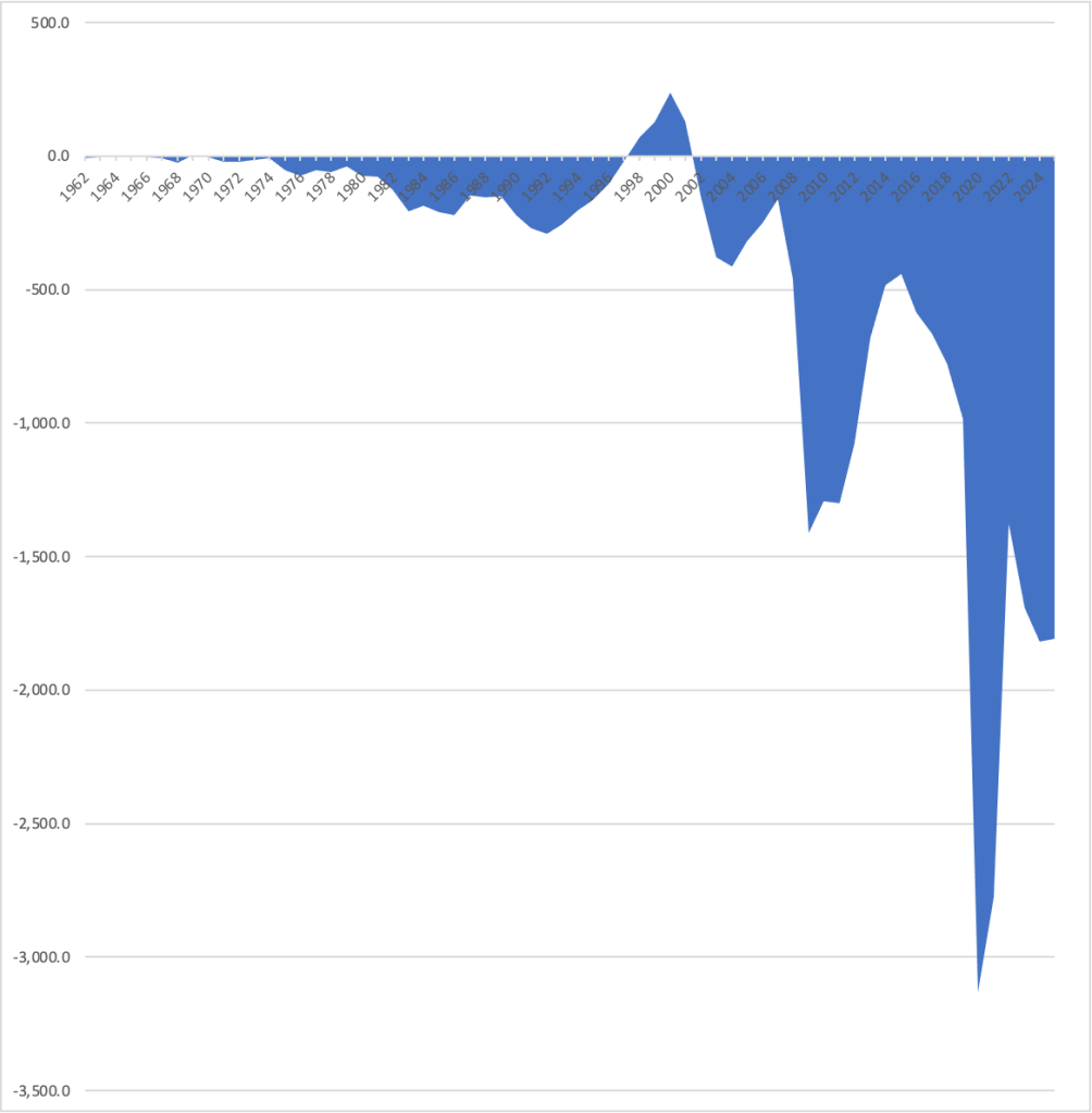
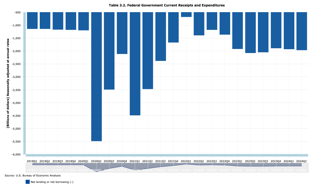
The federal government’s fiscal year runs from October 1 to September 30. Today (October 8), the Congressional Budget Office (CBO) released its estimate of the deficit for the fiscal year ending September 30, 2025. The deficit fell slightly from $1,817 billion in 2024 to $1,809 in 2025. As the following figure shows, the budget deficit in 2025 remains very large, particularly at a time when the U.S. economy is at or very close to full employment, although well below the record deficit of $3,133 billion in 2020.
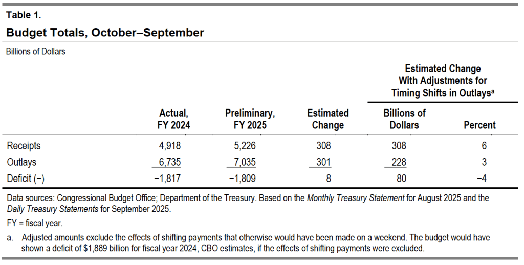
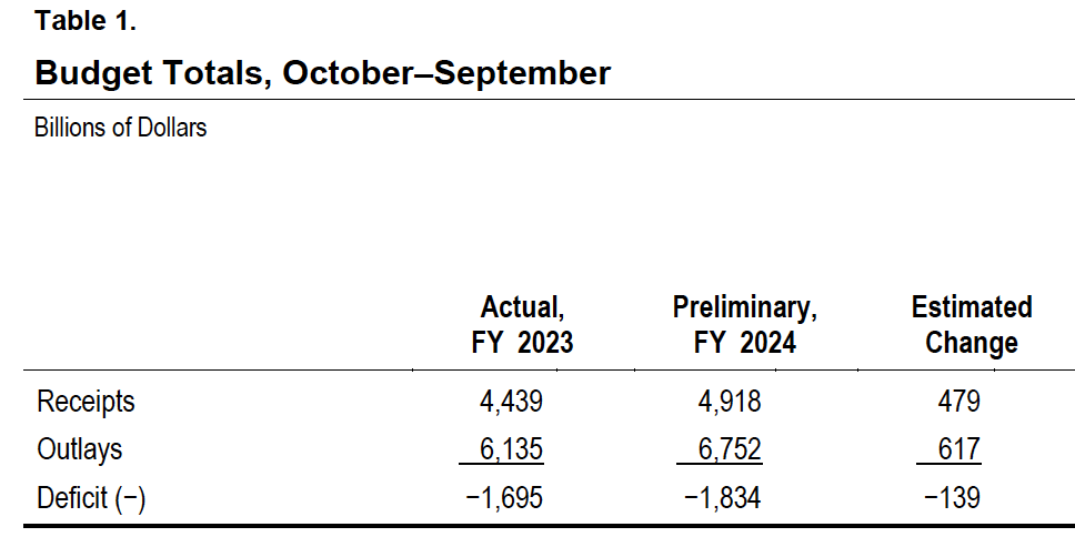
The following table from the CBO report shows that in 2025 federal receipts increased slightly more than federal outlays, leading to a slightly smaller deficit.
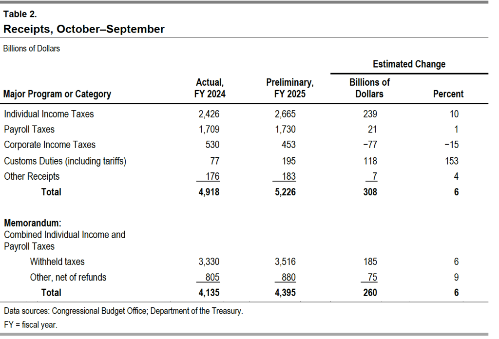
The next table shows the changes in the major categories of federal receipts. Individual income and payroll taxes—which fund the Social Security and Medicare programs, as well as the federal government’s contributions to state unemployment insurance plans—both increased, while corporate income tax receipts fell. The biggest change was in custom duties, which more than doubled following the Trump administration’s sharp increase in tariff rates beginning on April 2.
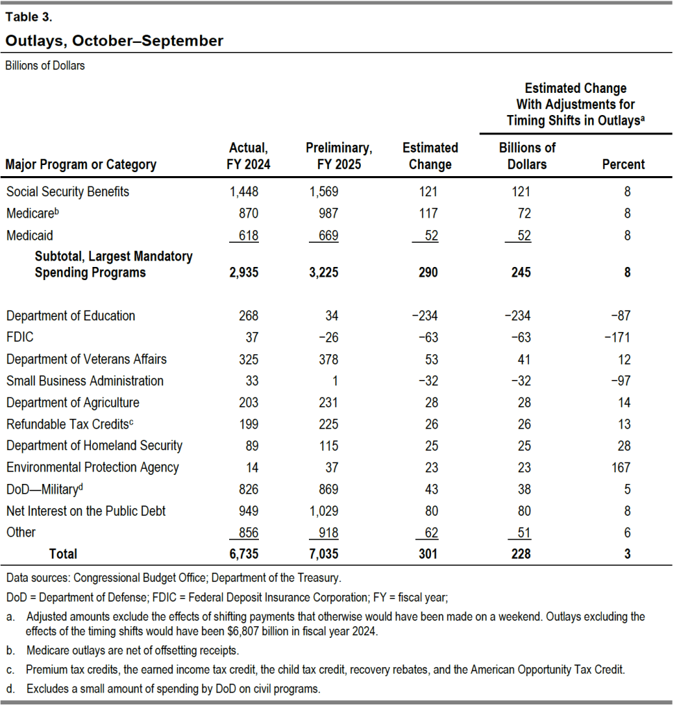
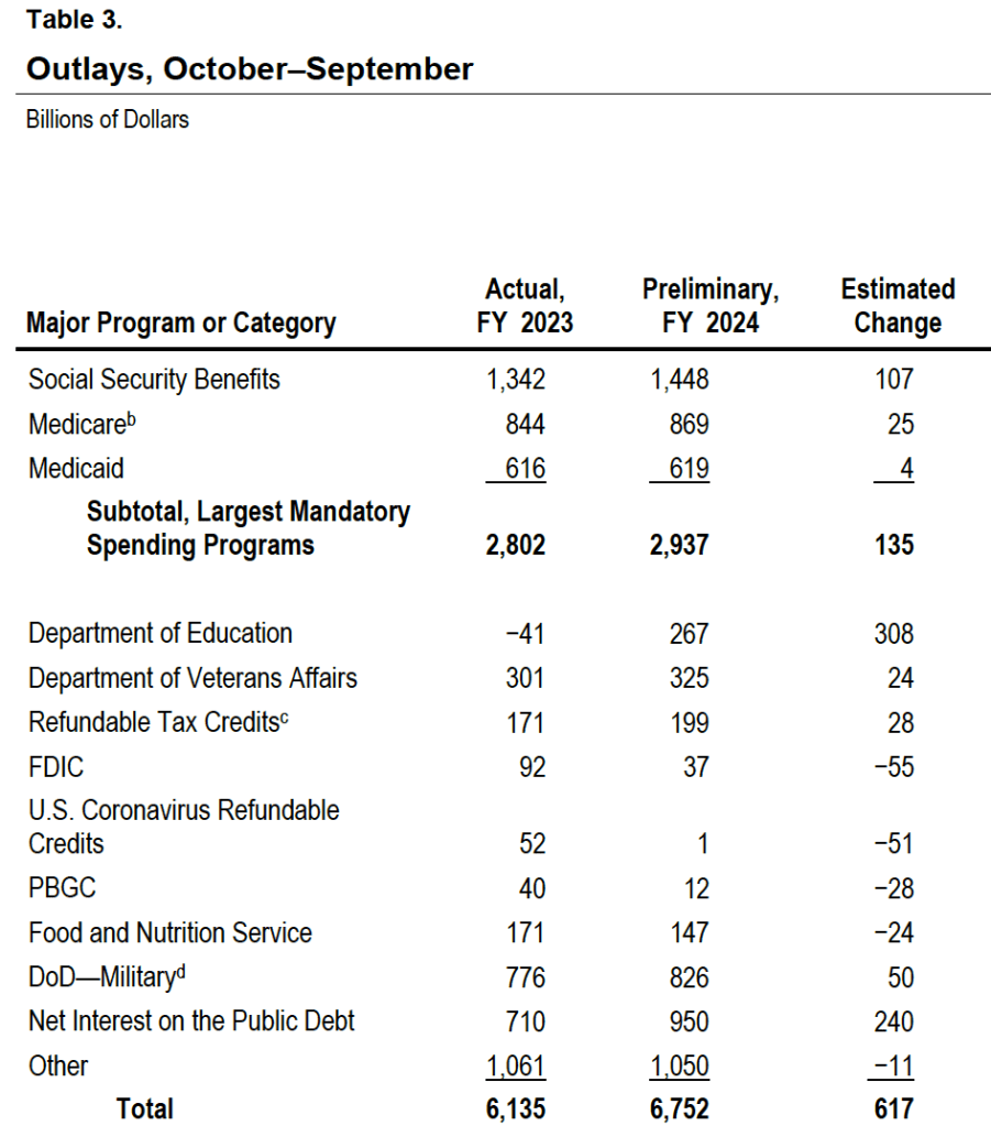
The next table shows the changes in the major categories of federal outlays. Spending on the Social Security, Medicare (health insurance for older people), and Medicaid (health insurance for lower-income people) programs continue to rapidly increase. Spending on Medicare is now more than $100 billion greater than spending on defense. Interest on the public debt continues to increase as the debt increases and interest rates remain well above their pre-2021 levels.
This morning (September 30), the federal government appears headed for a shutdown at midnight. As this handy explainer by David Wessel on the Brookings Institution website notes:
“… federal agencies cannot spend or obligate any money without an appropriation (or other approval) from Congress. When Congress fails to enact the 12 annual appropriation bills, federal agencies must cease all non-essential functions until Congress acts.
Government employees who provide what are deemed essential services, such as air traffic control and law enforcement, continue to work, but don’t get paid until Congress takes action to end the shutdown. All this applies only to the roughly 25% of federal spending subject to annual appropriation by Congress.”
A federal government shutdown can cause significant inconvenience to people who rely on nonessential government services. Federal government employees won’t receive paychecks nor will contractors supplying nonessential services, such as cleaning federal office buildings. Many federal government facilities, such as museums and national parks will be closed or will operate on reduced hours. It seems likely that the Bureau of Labor Statistics will not release on time its “Employment Situation Report” for September, which was due on Friday.
Apart from the effects just listed, how might a shutdown affect the broader economy? The most recent federal government shutdown occurred during the first Trump administration and lasted from December 22, 2018 to January 25, 2019. At the end of that shutdown, the Congressional Budget Office (CBO) prepared a report on its economic effects. The main conclusion of the report was that:
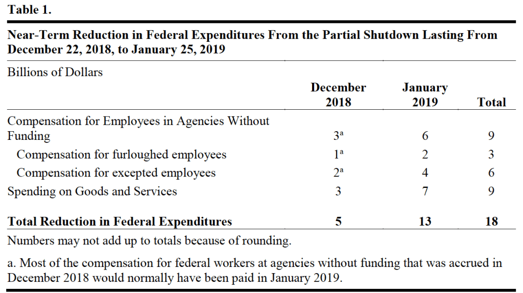
“In CBO’s estimation, the shutdown dampened economic activity mainly because of the loss of furloughed federal workers’ contribution to GDP, the delay in federal spending on goods and services, and the reduction in aggregate demand (which thereby dampened private-sector activity).”
Table 1 from the CBO report shows the effect of the shutdown on federal government expenditures. (Note that the CBO refers to the shutdown as being “partial” because, as in all federal government shutdowns, essential government services continued to be provided.)
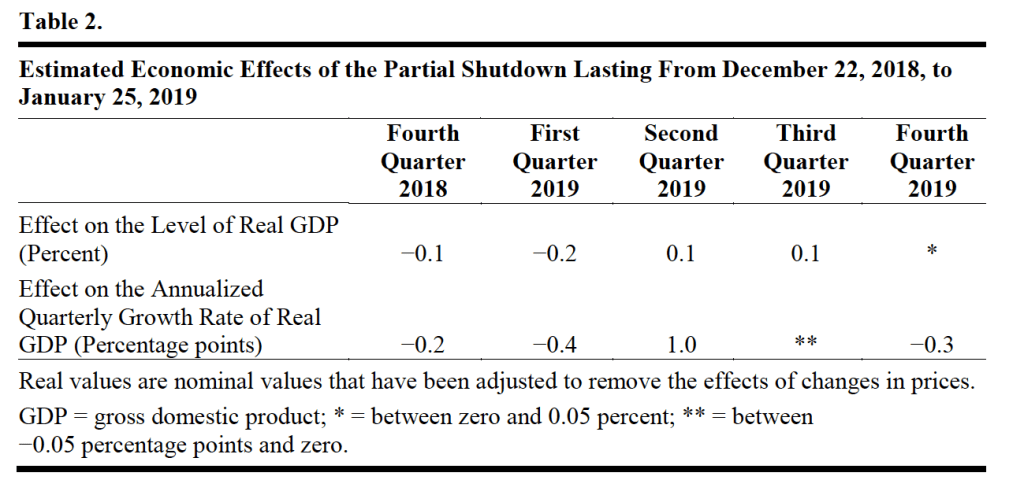
Table 2 from the report shows the effects of the shutdown on real GDP.
Most of the macroeconomic effects of a government shutdown aren’t long lasting because most federal government spending that doesn’t occur during the shutdown is postponed rather than eliminated. When federal government employees return to work after the shutdown, they typically receive backpay for the time they were furloughed. The CBO estimates that the lasting effect of the shutdown on GDP was small “about $3 billion in forgone economic activity will not be recovered. That amount equals 0.02 percent of projected annual GDP in 2019.”
Will a federal government shutdown that begins at midnight tonight and lasts for a few weeks also have only a short-lived effect on the economy? That seems likely, although the Trump administration has indicated that if a shutdown occurs, some federal government employees will be fired rather than just furloughed. A significant reduction in federal employment could lead to a larger decrease in GDP that might persist for longer. The effect on the areas of Virginia and Maryland where most federal government workers live could be significant in the short run.
In June, the U.S. Census Bureau released its population estimates for 2024. Included was the following graphic showing the change in the U.S. population pyramid from 2004 to 2024. As the graphic shows, people 65 years and older have increased as a fraction of the total population, while children have decreased as a fraction of the total population. (The Census considers everyone 17 and younger to be a child.) Between 2004 and 2024, people 65 and older increased from 12.4 percent of the population to 18.0 percent. People younger than 18 fell from 25.0 percent of the population in 2004 to 21.5 percent in 2024.
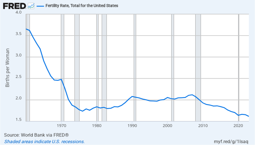
The aging of the U.S. population reflects falling birth rates. Demographers and economists typically measure birth rates as the total fertility rate (TFR), which is defined by the World Bank as: “The number of children that would be born to a woman if she were to live to the end of her childbearing years and bear children in accordance with age-specific fertility rates currently observed.” The TFR has the advantage over the simple birth rate—which is the number of live births per thousand people—because the TFR corrects for the age structure of a country’s female population. Leaving aside the effects of immigration and emigration, a TFR of 2.1 is necessary to keep a country’s population stable. Stated another way, a country needs a TFR of 2.1 to achieve replacement level fertility. A country with a TFR above 2.1 experiences long-run population growth, while a country with a TFR of less than 2.1 experiences long-run population decline.
The following figure shows the TFR for the United States for each year between 1960 and 2023. Since 1971, the TFR has been below 2.1 in every year except for 2006 and 2007. Immigration has helped to offset the effects on population growth of a TFR below 2.1.
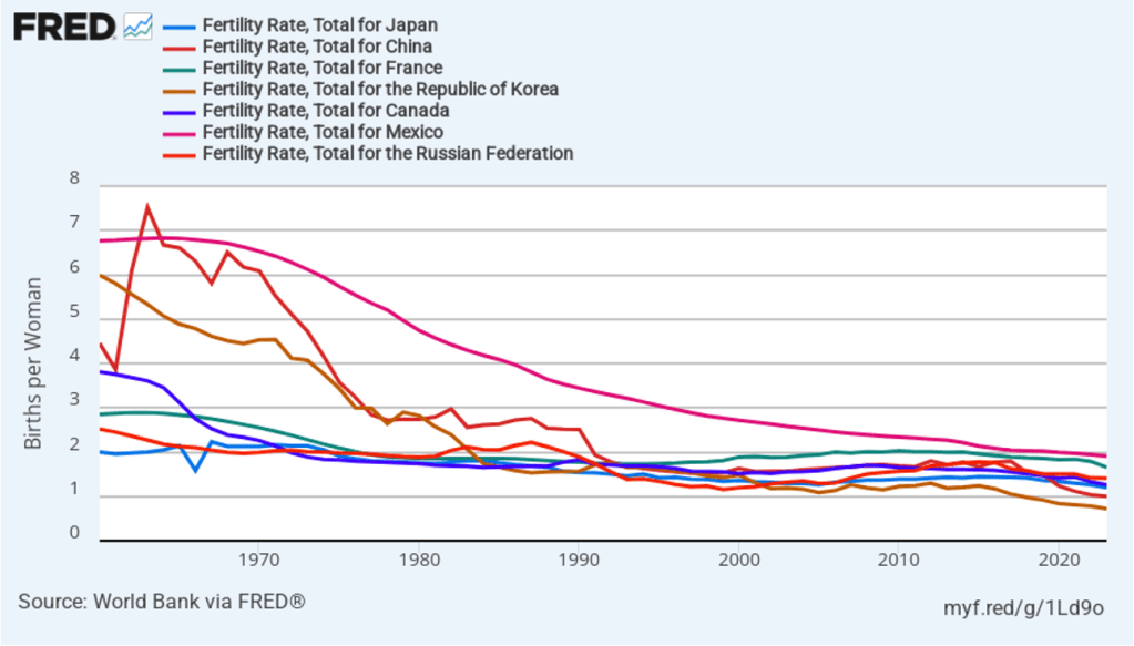
The United States is not alone in experiencing a sharp decline in its TFR since the 1960s. The following figure shows some other countries that currently have below replacement level fertility, including some countries—such as China, Japan, Korea, and Mexico—in which TFRs were well above 5 in the 1960s. In fact, only a relatively few countries, such as Israel and some countries in sub-Saharan Africa are still experiencing above replacement level fertility.
An aging population raises the number of retired people relative to the number of workers, making it difficult for governments to finance pensions and health care for older people. We discuss this problem with respect to the U.S. Social Security and Medicare programs in an Apply the Concept in Macroeconomics, Chapter 16 (Economics, Chapter 26 and Essentials of Economics, Chapter 18). Countries experiencing a declining population typically also experience lower rates of economic growth than do countries with growing populations. Finally, as we discuss in an Apply the Concept in Microeconomics, Chapter 3, different generations often differ in the mix of products they buy. For instance, a declining number of children results in declining demand for diapers, strollers, and toys.
Glenn, along with co-authors Douglas Elmendorf of Harvard’s Kennedy School and Zachary Liscow of the Yale Law School, has written a new National Bureau of Economic Research working paper: “Policies to Reduce Federal Budget Deficits by Increasing Economic Growth”
Here’s the abstract:
Could policy changes boost economic growth enough and at a low enough cost to meaningfully reduce federal budget deficits? We assess seven areas of economic policy: immigration of high-skilled workers, housing regulation, safety net programs, regulation of electricity transmission, government support for research and development, tax policy related to business investment, and permitting of infrastructure construction. We find that growth-enhancing policies almost certainly cannot stabilize federal debt on their own, but that such policies can reduce the explicit tax hikes, spending cuts, or both that are needed to stabilize debt. We also find a dearth of research on the likely impacts of potential growth-enhancing policies and on ways to design such policies to restrain federal debt, and we offer suggestions for ways to build a larger base of evidence.
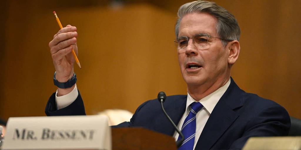
Treasury Secretary nominee Scott Bessent. (Photo from Progect Syndicate.)
By setting an ambitious 3% growth target, U.S. Treasury Secretary nominee Scott Bessent has provided the Trump administration a North Star to follow in devising its economic policies. The task now is to focus on productivity growth and avoiding any unforced errors that would threaten output.
U.S. Treasury Secretary nominee Scott Bessent is right to emphasize faster economic growth as a touchstone of Donald Trump’s second presidency. More robust growth not only implies higher incomes and living standards—surely the basic objective of economic policy—but also can reduce America’s yawning federal budget deficit and debt-to-GDP ratio, and ease the sometimes difficult trade-offs across defense, social, and education and research spending.
But faster growth must be more than just a wish. Achieving it calls for a carefully constructed agenda, based on a recognition of the channels through which economic policies can raise or reduce output. While a pro-investment tax policy might boost capital accumulation, productivity, and GDP, higher interest rates from deficit-financed tax or spending changes might have the opposite effect. Similarly, since growth in hours worked is a component of growth in output or GDP, the new administration should avoid anti-work policies that hinder full labor-force participation, as well as sudden adverse changes to legal immigration.
While recognizing that some policy shifts that increase output might adversely affect other areas of social interest (such as the distribution of income) or even national security, policymakers should focus squarely on increasing productivity. The three pillars of any productivity policy are support for research, investment-friendly tax provisions, and more efficient regulation.
Ideas drive prospects in modern economies. Basic research in the sciences, engineering, and medicine power the innovation that advances technology, improvements in business organization, and gains in health and well-being. It makes perfect sense for the federal government to support such research. Since private firms cannot appropriate all the gains from their own outlays for basic research, they have less of an incentive to invest in it. Moreover, government support in this area produces valuable spillovers, as demonstrated by the earlier Defense Department research expenditures that became catalysts for today’s digital revolution.
This being the case, cuts in federal support for basic research are inconsistent with a growth agenda. Still, policymakers should review how research funds are distributed to ensure scientific merit, and they should encourage a healthy dose of risk-taking on newer ideas and researchers.
In addition to encouraging commercialization of spillovers from basic research and defense programs, federal support for applied research centers around the country would accelerate the dissemination of new productivity-enhancing technologies and ideas. Such centers also tend to distribute the economy’s prosperity more widely, by making new ideas broadly accessible—as agricultural- and manufacturing-extension services have done historically.
To address the second pillar of productivity growth, the administration should seek to extend the pro-investment provisions of the Tax Cuts and Jobs Act that Trump signed into law in 2017. While the TCJA’s lower tax rates on corporate profits remain in place, the expensing of business investment – a potent tool for boosting capital accumulation, productivity, and incomes – was set to be phased out over the 2023-26 period. This provision could be restored and made permanent by reducing spending on credits under the Inflation Reduction Act, or by rolling back the spending – such as $175 billion to forgive student loans – associated with outgoing President Joe Biden’s executive orders.
If the new administration wanted to go further with tax policy, it could build on the 2016 House Republican blueprint for tax reform that shifted the business tax regime from an income tax to a cashflow tax. By permitting immediate expensing of investment, but not interest deductions for nonfinancial firms, this reform would stimulate investment and growth, remove tax incentives that favor debt over equity, and simplify the tax system.
That brings us to the third pillar of a successful growth strategy: efficient regulation. The issue is not “more” versus “less.” What really matters for growth is how changes in regulation can improve the prospects for growth through innovation, investment, and capital allocation, while focusing on trade-offs in risks. Those shaping the agenda should start with basic questions like: Why can’t we build better infrastructure faster? Why can’t capital markets and bank lending be nimbler? Not only do such questions identify a specific goal; they also require one to identify trade-offs.
Fortunately, financial regulation under the new administration is likely to improve capital allocation and the prospects for growth, given the leadership appointments already announced at the Securities and Exchange Commission and the Federal Reserve. But policymakers also will need to improve the climate for building infrastructure and enhancing the country’s electricity grids to support the data centers needed for generative artificial intelligence. This will require a sharper focus on cost-benefit analysis at the federal level, as well as better coordination with state and local authorities on permitting. Using federal financial support programs as carrots or sticks can be part of such a strategy.
Bessent’s emphasis on economic growth is spot on. By setting an ambitious 3% target for annual growth, he has provided the new administration a North Star to follow in devising its economic policies.
On January 5, 2025 at the American Economic Association meetings in San Francisco, Jason Furman of Harvard’s Kennedy School, former Federal Reserve Chair Ben Bernanke (now of the Brookings Institution), former Council of Economic Advisers Chair Christina Romer of the University of California, Berkeley, and John Cochrane of Stanford’s Hoover Institition participated in a panel on “Inflation and the Macroeconomy.”
The discussion provides an interesting overview of a number of macroeconomic topics including:
The roles of aggregate demand shocks and aggregate supply shocks in explaining the sharp increase of inflation beginning in the spring of 2021.
The reasons for the Fed’s delay in responding to the increase in inflation.
Why macroeconomic forecasting models and most economists failed to anticipate the rise in inflation.
The role of the Fed’s 2020 monetary policy framework, how the Fed should revise the framework as a result of the review currently underway, and whether the Fed should change its inflation target. (We discuss the Fed’s monetary policy framework in several blog posts, including this one.)
The likely future course of inflation and the potential effects of the Trump Administration’s policies.
The likely consequences of large federal budget deficits.
Threats to Fed independence.
The discussion is fairly long at two hours, but most of it is nontechnical and should be understandable by students who have reached the monetary and fiscal policy chapters of a macroeconomic principles course (Chapters 15 and 16 of Macroeconomics; Chapters 25 and 26 of Economics).
Image generated by GTP-4o illustrating labor productivity
Several articles in the business press have discussed the recent increases in labor productivity. For instance, this article appeared in this morning’s Wall Street Journal (a subscription may be required).
The most widely used measure of labor productivity is output per hour of work in the nonfarm business sector. The BLS calculates output in the nonfarm business sector by subtracting from GDP production in the agricultural, government, and nonprofit sectors. (The definitions used by the Bureau of Labor Statistics (BLS) in estimating labor productivity are discussed in the “Technical Notes” that appear at the end of the BLS’s quarterly “Productivity and Costs” releases.) The blue line in the following figure shows the annual growth rate in labor productivity in the nonfarm business sector as measured by the percentage change from the same quarter in the previous year. The green line shows labor productivity growth in manufacturing.
As the figure shows, both labor productivity growth in the nonfarm business sector and labor productivity growth in manufacturing are volatile. The business press has focused on the growth of productivity in the nonfarm business sector during the period from the third quarter of 2023 through the third quarter of 2024. During this time, labor productivity has grown at an average annual rate of 2.5 percent. That growth rate is notably higher than the growth rate that many economists are expecting over the next 10 years. For instance, the Congressional Budget Office (CBO) has forecast that labor productivity will grow at an average annual rate of only 1.6 percent over the period from 2025 to 2034.
The CBO forecasts that the total numbers of hours worked in the economy will grow at an average annual rate of 0.5 percent. Combining that estimate with a 2.5 percent annual rate of growth of labor productivity results in output per person—a measure of the standard of living—increasing by 34 percent by 2034. If labor productivity increases at a rate of only 1.6 percent, then output per person will have increased by only 23 percent by 2034.
The standard of living of the average person in United States increasing 11 percent more would make a noticeable difference in people’s lives by allowing them to consume and save more. Higher rates of labor productivity growth leading to a faster growth rate of income and output would also increase the federal government’s tax revenues, helping to decrease federal budget deficits that are currently forecast to be historically large. (We discuss the components of long-run economic growth in Macroeconomics, Chapter 16, Section 16.7; Economics, Chapter 26, Section 26.7, and the economics of long-run growth in Macroeconomics, Chapter 11; Economics, Chapter 21.)
Can the recent growth rates in labor productivity be maintained over the next 10 years? There is an historical precedent. Labor productivity in the nonfarm business sector grew at an average annual rate of 2.6 percent between 1950 and 1973. But growth rates that high have proven difficult to achieve in more recent years. For instance, from 2008 to 2023, labor productivity grew at an average annual rate of only 1.5 percent. (We discuss the debate over future growth rates in Macroeconomics, Chapter 11, Section 11.3; Economics, Chapter 21, Section 21.3.)
The Wall Street Journal article we cited earlier provides an overview of some of the factors that may account for the recent increase in labor productivity growth rates. The 2020 Covid pandemic may have led to some increases in labor productivity. Workers who temporarily or permanently lost their jobs as businesses closed during the height of the pandemic may have found new jobs that better matched their skills, making them more productive. Similarly, businesses that were forced to operate with fewer workers, may have found ways to restore their previous levels of output with lower levels of employment. These changes may have led to one-time increases in labor productivity at some firms, but are unlikely to result in increased rates of labor productivity growth in the future.
Some businesses have used newly available generative artificial intelligence (AI) software to increase labor productivity by, for instance, using software to replace workers who previously produced marketing materials or responded to customer questions or complaints. It will take at least several years before generative AI software spreads throughout the economy, so it seems too early for it to have had a broad enough effect on the economy to be visible in the productivity data.
Note also that, as the green line in the figure above shows, manufacturing productivity has been lagging recently. From the third quarter of 2023 to the third quarter of 2024, labor productivity in manufacturing has increased at an annual average rate of only 0.4 percent. This slowdown is surprising given that over the long run productivity in manufacturing has typically increased faster than has productivity in the overall economy. It seems unlikely that labor productivity in the overall economy can sustain its recent growth rates if labor productivity growth in manufacturing continues to lag.
Finally, the productivity data are subject to revision as better estimates of output and of hours worked become available. It’s possible that what appear to be rapid rates of productivity growth during the last five quarters may turn out to have been less rapid following data revisions.
So, while the recent increase in the growth rate of labor productivity is an encouraging sign of the strength of the U.S. economy, it’s too soon to tell whether we have entered a sustained period of higher productivity growth.
Image showing scientific research generated by GTP-4o
Note: The following op-ed first appeared in the Wall Street Journal.
The Trump Economic Awakening
Traditional policies like tax cuts, targeted aid and responsible spending can deliver stronger growth.
Political scientists will debate the forces that shaped Donald Trump’s victory, but one thing is clear: Americans yearn for a change in economic policy. Voters have rejected the interventionist policies that brought inflation and high deficits. They want an economic awakening, a new way forward that uses traditional economic policies to achieve Mr. Trump’s goal of more jobs for Americans whose fortunes have been harmed by technological change and globalization.
Any economic path to a successful awakening begins with growth: the engine that powers individual income and our collective ability to support the nation’s defense, economy, education and healthcare industry. To pursue this growth, the new administration should consider at least three measures:
First, by working with Congress, it should build on the successes of the Tax Cuts and Jobs Act of 2017 to make permanent the expensing of business investment. Second, it should increase support for science and defense research, which would have significant spillover to the commercial sector, particularly in space exploration. Third, it should build on this research by constructing applied research centers around the country, linked to regional university and city hubs. Like the land-grant colleges of the 19th century, these centers would generate and distribute knowledge, improving local capabilities in manufacturing and services.
Opportunity is also a pillar of the awakening. Community colleges are an underfunded source of skill-building and mobility. As Austan Goolsbee, Amy Ganz and I proposed in a 2019 report, a modest federal block grant to support community colleges on the supply side—rather than a demand-side emphasis on financial aid—can help these schools push more Americans toward better jobs by working with local employers on skill needs and curriculum development. Targeted aid to places with depressed economic activity can help distribute opportunity to communities better than one-size-fits-all Washington-directed programs.
Corporate tax reform can play a role, too, by improving incentives for companies to settle and invest in the U.S. This can magnify opportunities for Americans, all without having to rely on costly tariffs.
Working a job doesn’t merely generate income; it also promotes human dignity. Enlisting more people into the workforce is thus another element of the economic-policy awakening. While growth and opportunity policies can boost labor-force participation, strengthening the earned-income tax credit to boost the incomes of childless workers can help attract younger people to the workforce. Maintaining the child tax credit can also provide parents with easier pathways toward economic participation.
These ideas share several important themes with Mr. Trump’s campaign and the traditional conservative playbook. They emphasize that policy ideas should be practical and workable, not merely rhetorical. Each makes use of America’s federalist system and innovative ethos. Making a priority of strong local involvement in applied research centers and community colleges and as tailoring place-based aid are more effective approaches than Washington diktats. Programs need to be held accountable for results, not simply allocated money.
This economic-policy awakening requires a clear-eyed assessment of budget trade-offs. Profligate spending with little regard for debt and inflation—à la the American Rescue Plan—contributed to Mr. Trump’s victory. It is possible to accomplish the steps above in a fiscally responsible way by offsetting spending and tax changes.
Organizing for the policy awakening’s success will be essential. Lack of communication among cabinet agencies can stymie creative ideas for expanding the economic pie for American workers. Like the president’s Working Group on Financial Markets, created by Ronald Reagan in 1988 to convene disparate agencies, the new administration would benefit from a senior executive team that can coordinate economic ideas and learn from leaders in business, labor and social services. Such a body, unlike the National Economic Council, could more adeptly cut across silos related to tax, trade, regulatory and industrial policy.
Voters have signaled they’re ready for an economic awakening. The president-elect, equipped with a new playbook and vision, should seize the opportunity.
Logo of the Congressional Budget Office from cbo.gov.
The federal government’s fiscal year runs from October 1 to September 30 of the following calendar year. The Congressional Budget Office (CBO) estimates that the federal government’s budget deficit for fiscal 2024, which just ended, was $1.8 trillion. (The Office of Management and Budget (OMB) will release the official data on the budget later this month.)
The federal budget deficit increased by about $100 billion from fiscal 2023, although the comparison of the deficits in the two years is complicated by the question of how to account for the $333 billion in student debt cancellation that President Biden ordered (which would reduce federal revenues by that amount) but which wasn’t implemented because of a decision by the U.S. Supreme Court.
The following table from the CBO report compares federal receipts and outlays for fiscal years 2023 and 2024. Recipts increased by $479 billion from 2023 to 2024, but outlays increased by $617 billion, resulting in an increase of $139 billion in the federal budget deficit.
The following table shows the increases in the major spending categories in the federal budget. Spending on the Social Security, Medicare, and Medicaid programs increased by a total of $135 billion. The large increase in spending on the Department of Education is distorted by accounting for the reversal of the student debt cancellation following a Suprement Court ruling, as previously mentioned. The FDIC is the Federal Deposit Insurance Corporation, which had larger than normal expenditures in 2023 due the failure of several regional banks. (We discuss this episode in several earlier blog posts, including this one.) Interest on the public debt increased by $240 billion because of increases in the debt as a result of persistently high federal deficits and because of increases in the interest rates the Treasury has paid on new issues of bill, notes, and bonds necessary to fund those deficits. (We discuss the federal budget deficit and federal debt in Macroeconomics, Chapter 16, Section 16.6 (Economics, Chapter 26, Section 26.6).)
A troubling aspect of the large federal budget deficits is that they are occurring during a time of economic expansion when the economy is at full employment. The following figure, using data from the Bureau of Economic Analysis (BEA), shows that at an annual rate, the federal budget deficit has beening running between $1.9 trillion and $2.1 trillion each quarter since the first quarter of 2023, well after most of the federal spending increases to meet the Covid pandemic ended.
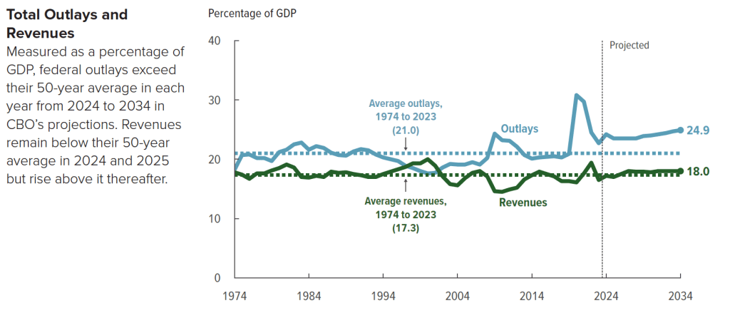
The following figure from the CBO shows trends in federal revenue and spending. From 1974 to 2023, federal spending averaged 21.o percent of GDP, but is forecast to rise to 24.9 percent of GDP by 2023. Federal revenue averaged 17.3 percent of GDP from 1974 to 2023 and is forecast to rise to 18.0 percent of GDP in 2034. As a result, the federal budget deficit, which had averaged 3.7 percent of GDP between 1974 and 2023 (already high in a longer historical context) will nearly double to 6.9 percent of GDP in 2034.
Slowing the growth of federal spending may prove difficult politically because the majority of spending increases are from manadatory spending on Social Security and Medicare, and from interest on the debt. Discretionary outlays are scheduled to decline in future years according to current law, but may well also increase if Congress and future presidents increase defense spending to meet the foreign challenges the country faces.
One possible course of future policy that would result in smaller future federal deficits is outlined in this post and the material at the included links.
Glenn serves on the the Grand Bargain Committee, chaired by Michael Strain of the American Enterprise Institute and Isabel Sawhill of the Brookings Institution. The committee, whose members span the political spectrum, have prepared a report that addresses some of the country’s most pressing economic and social problems.
Glenn and Michael Strain prepared the following introduction to the report. Below there is a link to the whole report.
The views expressed in this report are those of the individual authors who collectively constitute the Grand Bargain Committee, co-chaired by Michael R. Strain and Isabel V. Sawhill. This report was sponsored by the Center for Collaborative Democracy and was prepared independent of influence from the center and from any other outside party or institution. It is being published by the Bipartisan Policy Center as an example of how people with diverse views and political leanings can find common ground. The recommendations are strictly those of the policy experts and do not necessarily reflect the views of any organization or those of the BPC. All data are current as of November 2023.
By: Eric Hanushek, G. William Hoagland, Douglas Holtz-Eakin, R. Glenn Hubbard, Maya MacGuineas, Richard V. Reeves, Robert D. Resichauer, Gerard Robinson, Isabel V. Sawhill, Diane Schanzenbach, Richard Schmalensee, Michael R. Strain, and C. Eugene Steuerle.
Introduction
The United States faces serious economic and social challenges, including:
The underlying economic growth rate has slowed, as have opportunities for people to move up the economic ladder.
Our education system fails too many children and leaves many more with fewer opportunities than they deserve.
The nation is not rising to the challenge of addressing climate change.
Both our health care system and the health of our population need improvement.
Our income tax system is broken, generating tax revenue in an inefficient and unfair manner.
And the national debt is growing at an unsustainable pace, threatening long-term economic growth, crowding out needed investments in economic opportunity, and placing the nation’s ability to respond to a future crisis at risk.
To address these problems, the Center for Collaborative Democracy commissioned subject matter experts—progressives, centrists, and conservatives—to develop a “Grand Bargain” encompassing all six issues. The policy debate typically puts these problems into silos, and within each silo, powerful forces support the status quo. This report seeks to break down these silos. Dealing with them all at once—in a Grand Bargain—is a more promising strategy than dealing with them individually, because it allows for different parties to strike deals across policy issues, not just within a single issue.
For example, implementing a carbon tax to address climate change seems impossibly difficult. So does increasing accountability for teacher performance. Trading one for the other might be easier than pursuing both in isolation. Fixing the structural budget deficit by reducing entitlement spending is an enormous political challenge. So is increasing spending on programs that advance economic opportunity. Doing both at the same time could be more politically feasible than addressing them separately.
In this context, the group of experts met for several months in 2023 to share perspectives and ideas and to come up with sensible policies in each of these areas: economic growth and mobility; education; environment; health; taxes; and the federal budget. The end result is this report, which is being published by the Bipartisan Policy Center as an example of how people with diverse views and political leanings can find common ground.
This report is short, consisting of less than 30 pages of text. Its brevity is by design. This constraint forced the group to stay focused on issues and recommendations that matter the most. The focus of the report is on concepts. It is designed to answer such questions as, “How should the nation’s approach to education or to the federal budget change? What fundamental reforms are required to increase the underlying rates of economic growth and upward mobility?” Focusing on concepts means not focusing on policy details, including the details of implementing our recommendations and of transitioning across policy regimes. Our lack of attention to policy details does not mean we do not recognize their importance. Of course, we do, and many members of the group have spent much of their careers studying and designing public policies. Instead, we focus on concepts because we believe the United States needs to return to a discussion of first principles. This report advances that objective.
Not every member of the group agrees with every recommendation in this report. That is not surprising given the diversity of views in the group, and the difficulty and complexity of many of the issues we address. Despite this disagreement, we were able to have an informed and constructive discussion about these economic issues, to find compromises, and to come up with a set of recommendations that we believe, on balance, would greatly strengthen the country and improve people’s lives.
We believe in the importance of a market economy. Free markets have led to unprecedented growth and innovation, along with rising incomes, over the past three centuries. But government also has a role to play. To unleash more growth, we need to curtail unneeded or overly costly regulations and to create a tax system that encourages investment spending and innovation. To bring prosperity to more people, we need policies that will enable more people to benefit from economic growth through investment in their education and skills. For this reason, we put a great deal of emphasis on improving education for children, on training or retraining for adult workers, and on subsidizing the earnings of low-wage workers when necessary while maintaining a safety net for those who cannot work.
Our proposals are designed to advance certain underlying values and themes: Work and savings should be rewarded, investment should be encouraged over consumption, public assistance should be better targeted to those most in need, the tax system should be more progressive, and the nation should invest relatively more in the young and spend relatively less on the elderly.
Our specific proposals in each area are as follows:
On economic growth and mobility, we recommend investing in the education and training of workers, through community colleges and apprenticeships. We call for a more skill-based immigration system and for more immigrants; for encouraging innovation by investing more in basic research; for reducing taxes on new investment; for curbing unneeded regulation; for reducing the national debt; and for encouraging participation in economic life by increasing the generosity of earnings subsidies for low-wage workers.
On education, we recommend improving the teacher workforce at the K-12 level; paying teachers more but strengthening the link between pay and performance; maintaining educational standards and accountability while narrowing gaps by race and class; expanding school choice; and recognizing the role that parents and families must play in students’ learning.
On the environment, our main recommendation is to adopt a carbon tax. We also call for reducing methane emissions; expanding federal authority in the planning, siting, and permitting of the national electric transmission system; and repealing the renewable fuel standard that requires refiners to blend corn ethanol into the fuel they sell.
On health, we call for giving more attention to the social determinants of poor health with a focus on the need for better nutrition, for rationalizing existing subsidies for health care, and for reducing health care costs.
On taxes, we call for increasing tax revenue as a share of annual gross domestic product (GDP), and for that revenue to be raised in a manner that is more progressive, efficient, and simple than under current law, while also increasing the incentive to save and invest. For the business sector, that means allowing the expensing of investment expenditures and moving toward equal treatment of the corporate and noncorporate sectors.
On the federal budget, we recommend putting the debt as a share of annual GDP on a sustainable trajectory with a comprehensive package of reforms made up of a rough balance between tax increases and spending cuts in the initial years, phasing into a much larger share of the savings coming from spending cuts over time.
Most of these recommendations are at the federal level, but some are at the state and local level, particularly our education recommendations.
In the spirit of a Grand Bargain, these recommendations advance common goals and values through compromises both within and across policy areas. For example, one of our values is reflected in the goal of refocusing government spending on those who truly need it, and another is to restore fiscal responsibility. To accomplish this, we call for slower growth in Social Security and Medicare benefits for affluent seniors to reduce the major driver of the national debt, but we also protect vulnerable seniors and spend more on the education of children and on earnings subsidies for the working poor. We recommend adopting a carbon tax because it will simultaneously advance our goals of supporting the environment, increasing tax revenue, and boosting dynamism by encouraging innovation in the energy sector.
We believe the analysis and recommendations in this report point a path forward for the nation, but we offer them in a spirit of humility, understanding that others will disagree. We hope that this report catalyzes a much needed debate about the future of our nation.