Has the Federal Reserve Achieved a Soft Landing?

The Federal Reserve building in Washington, DC. (Photo from the New York Times.)

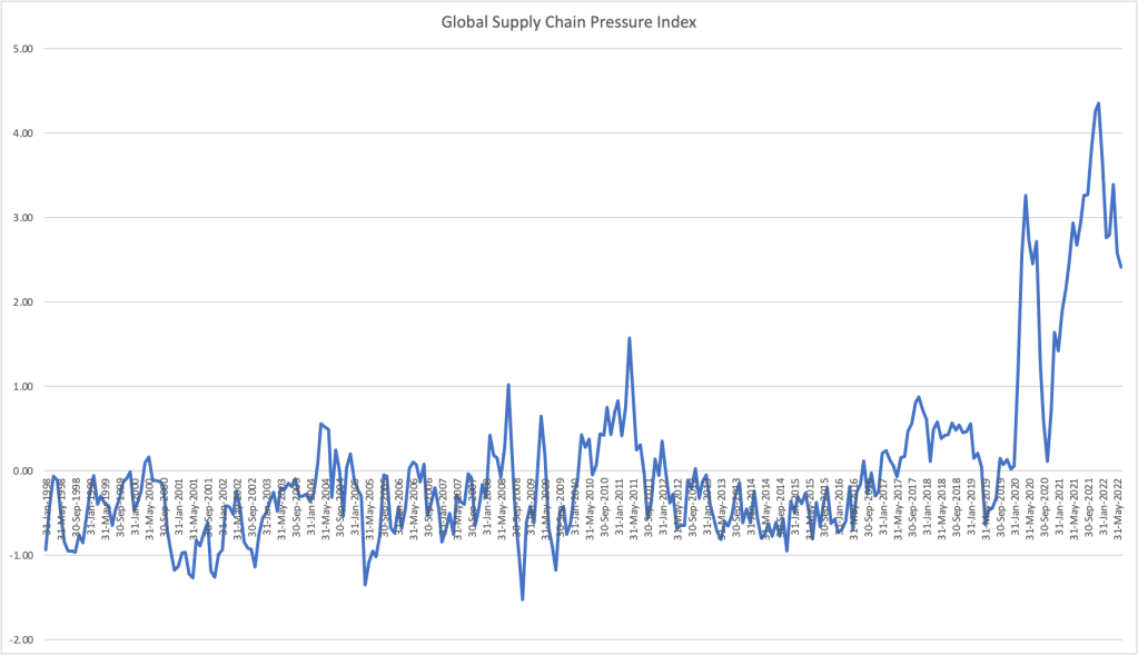
Since inflation began to increase rapidly in the late spring of 2021, the key macroeconomic question has been whether the Fed would be able to achieve a soft landing—pushing inflation back to its 2 percent target without causing a recession. The majority of the members of the Fed’s Federal Open Market Committee (FOMC) believed that increases in inflation during 2021 were largely caused by problems with supply chains resulting from the effects of the Covid–19 pandemic. 

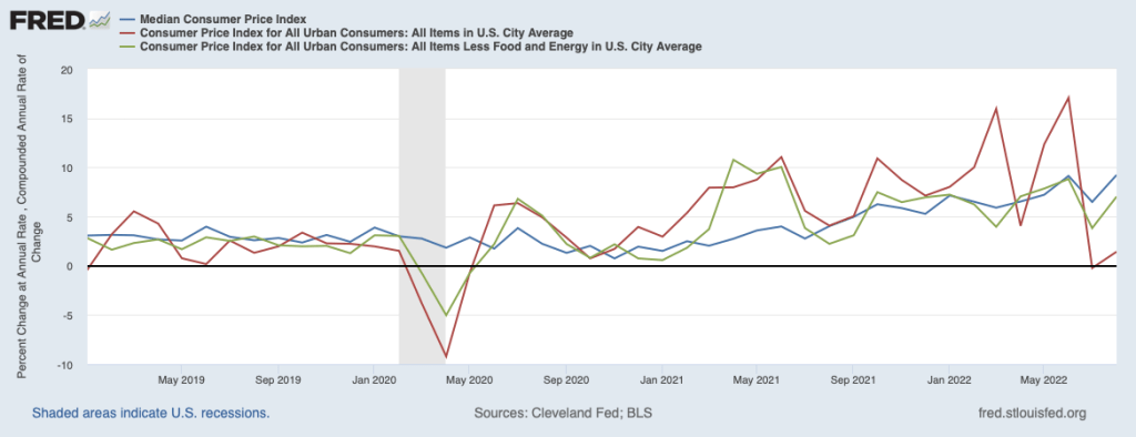
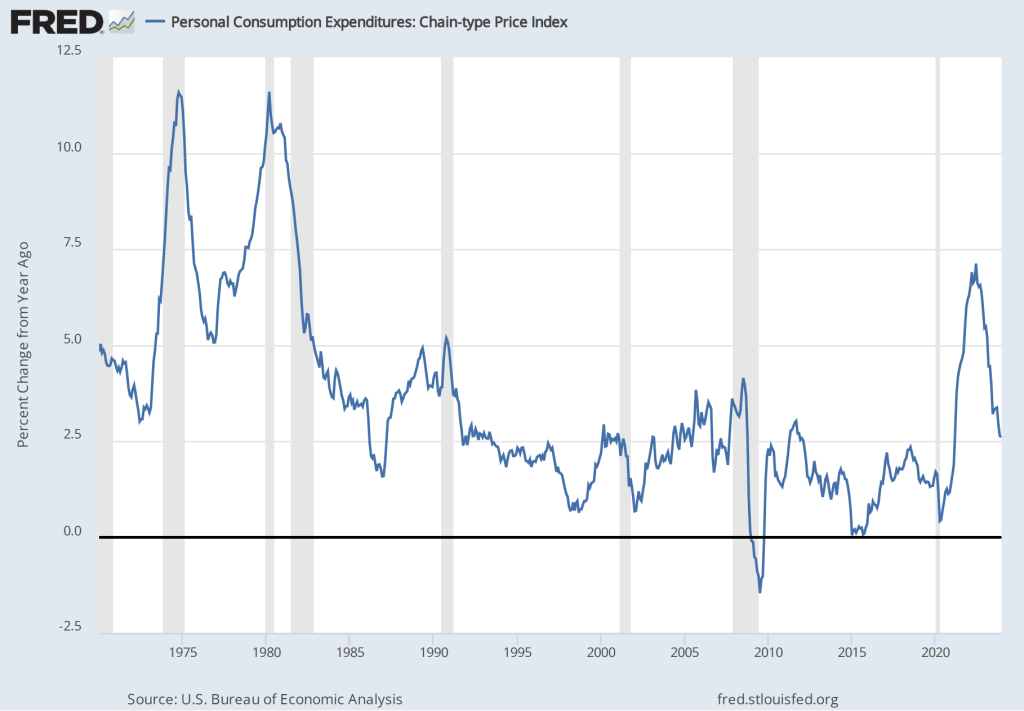
These committee members believed that once supply chains returned to normal, the increase in he inflation rate would prove to have been transitory—meaning that the inflation rate would decline without the need for the FOMC to pursue a contractionary monetary by substantially raising its target range for the federal funds rate. Accordingly, the FOMC left its target range unchanged at 0 to 0.25 percent until March 2022. As the following figure shows, by that time the inflation rate had increased to 6.9 percent, the highest it had been since January 1982. (Note that the figure shows inflation as measured by the percentage change from the same month in the previous year in the personal consumption expenditures (PCE) price index. Inflation as measured by the PCE is the gauge the Fed uses to determine whether it is achieving its goal of 2 percent inflation.)

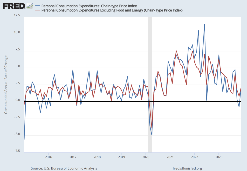
By the time inflation reached its peak in mid-2022, many economists believed that the FOMC’s decision to delay increasing the federal funds rate until March 2022 had made it unlikely that the Fed could return inflation to 2 percent without causing a recession.  But the latest macroeconomic data indicate that—contrary to that expectation—the Fed does appear to have come very close to achieving a soft landing.  On January 26, the Bureau of Economic Analysis (BEA) released data on the PCE for December 2023. The following figure shows for the period since 2015, inflation as measured by the percentage change in the PCE from the same month in the previous year (the blue line) and as measured by the percentage change in the core PCE, which excludes the prices of food and energy (the red line).  

The figure shows that PCE inflation continued its decline, falling slightly in December to 2.6 percent. Core PCE inflation also declined in December to 2.9 percent from 3.2 percent in November. Note that both measures remained somewhat above the Fed’s inflation target of 2 percent.

If we look at the 1-month inflation rate—that is the annual inflation rate calculated by compounding the current month’s rate over an entire year—inflation is closer to Fed’s target, as the following figure shows. The 1-month PCE inflation rate has moved somewhat erratically, but has generally trended down since mid-2022. In December, PCE inflation increased from from –0.8 percent in November (which acutally indicates that deflation occurred that month) to 2.0 percent in December. The 1-month core PCE inflation rate has moved less erratically, also trending down since mid-2022. In December, the 1-month core PCE inflation increased from 0.8 percent in November to 2.1 percent in December. In other words, the December reading on inflation indicates that inflation is very close to the Fed’s target.

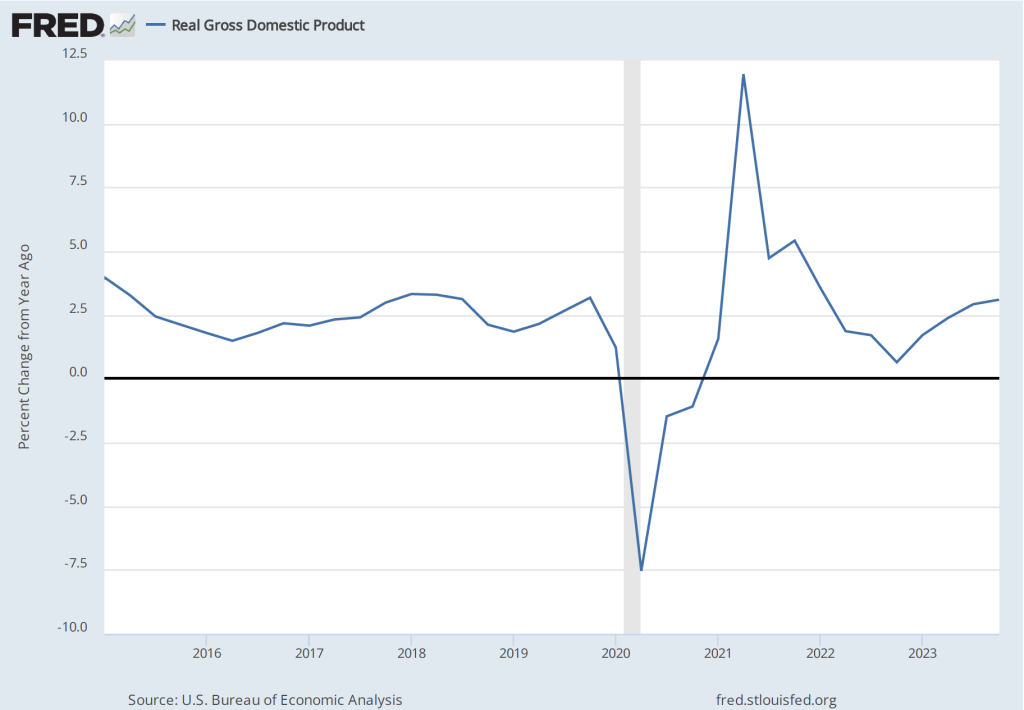
The following figure shows for each quarter since the beginning of 2015, the growth rate of real GDP measured as the percentage change from the same quarter in the previous year. The figure indicates that although real GDP growth dropped to below 1 percent in the fourth quarter of 2022, the growth rate rose during each quarter of 2023. The growth rate of 3.1 percent in the fourth quarter of 2023 remained well above the FOMC’s 1.8 percent estimate of long-run economic growth. (The average of the members of the FOMC’s estimates of the long-run growth rate of real GDP can be found here.) To this point, there is no indication from the GDP data that the U.S. economy is in danger of experiencing a recession in the near future.

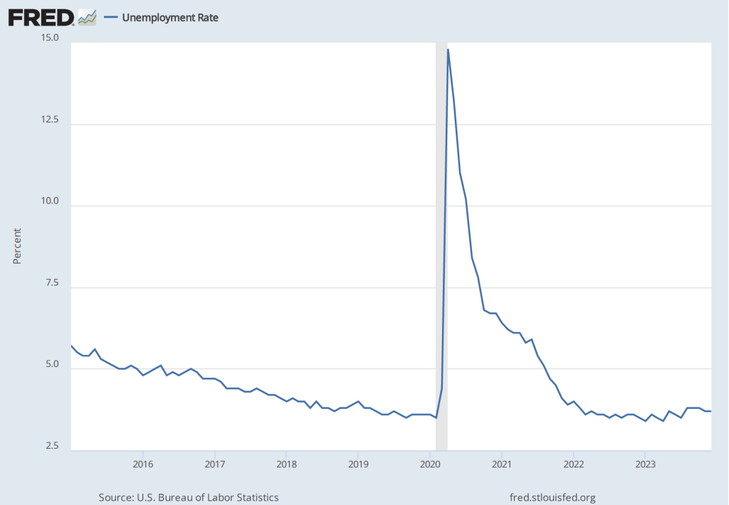
The labor market also shows few signs of a recession, as indicated by the following figure, which shows the unemployment rate in the months since January 2015. The unemployment rate has remained below 4 percent in each month since December 2021. The unemployment rate was 3.7 percent in December 2023, below the FOMC’s projection of a long-run unemployment rate of 4.1 percent.

The FOMC’s next meeting is on Tuesday and Wednesday of this week (February 1-2). Should we expect that at that meeting Fed Chair Jerome Powell will declare that the Fed has succeeded in achieving a soft landing? That seems unlikely. Powell and the other members of the committee have made clear that they will be cautious in interpreting the most recent macroeconomic data. With the growth rate of real GDP remaining above its long run trend and the unemployment rate remaining below most estimates of the natural rate of unemployment, there is still the potential that aggregate demand will increase at a rate that might cause the inflation rate to once again rise.

In a speech at the Brookings Institution on January 16, Fed Governor Christopher Waller echoed what appear to be the views of most members of the FOMC:

“Time will tell whether inflation can be sustained on its recent path and allow us to conclude that we have achieved the FOMC’s price-stability goal. Time will tell if this can happen while the labor market still performs above expectations. The data we have received the last few months is allowing the Committee to consider cutting the policy rate in 2024. However, concerns about the sustainability of these data trends requires changes in the path of policy to be carefully calibrated and not rushed. In the end, I am feeling more confident that the economy can continue along its current trajectory.”

At his press conference on February 1, following the FOMC meeting, Chair Powell will likely provide more insight into the committee’s current thinking.

Should the Fed Be Looking at the Median CPI?

For years, all the products for sale in Dollar Tree stores had a price of $1.00 or less. But as inflation increased, the company had to raise its maxium prices to $1.25. (Thanks to Lena Buonanno for sending us the photo.)

There are multiple ways to measure inflation. Economists and policymakers use different measures of inflation depending on the use they intend to put the measure of inflation to. For example, as we discuss in Macroeconomics, Chapter 9, Section 9.4 (Economics, Chapter 19, Section 19.4), the Bureau of Labor Statistics (BLS) constructs the consumer price index (CPI) as measure of the cost of living of a typical urban household. So the BLS intends the percentage change in the CPI to measure inflation in the cost of living as experienced by the roughly 93 percent of the population that lives in an urban household. (We are referring here to what the BLS labels CPI–U. As we discuss in this blog post, the BLS also compiles a CPI for urban wage earners and clerical workers (or CPI–W).)

As we discuss in an Apply the Concept in Chapter 15, Section 15.5, because the Fed is charged by Congress with ensuring stability in the general price level, the Fed is interested in a broader measure of inflation than the CPI. So its preferred measure of inflation is the personal consumption expenditures (PCE) price index, which the Bureau of Economic Analysis (BEA) issues monthly. The PCE price index is a measure of the price level similar to the GDP deflator, except it includes only the prices of goods and services from the consumption category of GDP. Because the PCE price index includes more goods and services than the CPI, it is suits the Fed’s need for a broader measure of inflation. The Fed uses changes in the PCE to evaluate whether it’s meeting its target of a 2 percent annual inflation rate.

In using either the percentage change in the CPI or the percentage change in the PCE, we are looking at what inflation has been over the previous year. But economists and policymakers are also looking for indications of what inflation may be in the future. Prices of food and energy are particularly volatile, so the BLS issues data on the CPI excluding food and energy prices and the BEA does the same with respect to the PCE. These two measures help avoid the problem that, for example, a period of high gasoline prices might lead the inflation rate to temporarily increase. Note that inflation caclulated by excluding the prices of food and energy is called core inflation.

During the surge in inflation that began in the spring of 2021 and continued into the fall of 2022, some economists noted that supply chain problems and other effects of the pandemic on labor and product markets caused the prices of some goods and services to spike. For example, a shortage of computer chips led to a reduction in the supply of new cars and sharp increases in car prices. As with temporary spikes in prices of energy and food, spikes resulting from supply chain problems and other effects of the pandemic might lead the CPI and PCE—even excluding food and energy prices—to give a misleading measure of the underlying rate of inflation in the economy. 

To correct for this problem, some economists have been more attention to the measure of inflation calculated using the median CPI, which is compiled monthly by economists at the Federal Reserve Bank of Cleveland. The median CPI is calculated by ranking the price changes of every good or service in the index from the largest price change to the smallest price change, and then choosing the price change in the middle. The idea is to eliminate the effect on measured inflation of any short-lived events that cause the prices of some goods and services to be particularly high or particularly low. Economists at the Cleveland Fed have conducted research that shows that, in their words, “the median CPI provides a better signal of the underlying inflation trend than either the all-items CPI or the CPI excluding food and energy. The median CPI is even better at forecasting PCE inflation in the near and longer term than the core PCE price index.”

The following figure shows the three measures of inflation using the CPI for each month since January 2019. The red line shows the unadjusted CPI, the green line shows the CPI excluding food and energy prices, and the blue line shows median CPI. To focus on the inflation rate in a particular month, in this figure we calculate inflation as the percentage change in the index at an annual rate. That is, we calculate the annual inflation rate assuming that the inflation rate in that month continued for a year.

Note that for most of the period since early 2021, during which the inflation rate accelerated, median inflation was well below inflation measured by changes in the unadjusted CPI. That difference reflects some of the distortions in measuring inflation arising from the effects of the pandemic.

But the last two values—for July and August 2022—tell a different story. In those months, inflation measured by changes in the CPI excluding food and energy prices or by changes in median CPI were well above inflation measured by changes in the unadjusted CPI.  In August 2022, the unadjusted CPI shows a low rate of inflation—1.4 percent—whereas the CPI excluding food and energy prices shows an inflation rate of 7.0 percent and the median CPI shows an inflation rate of 9.2 percent. 

We should always be cautious when interpreting any economic data for a period as short as two months. But data for inflation measured by the change in median CPI may be sending a signal that the slowdown in inflation that many economists and policymakers had been predicting would occur in the summer of 2022 isn’t actually occurring. We’ll have to await the release of future data to draw a firmer conclusion.

Sources: Michael S. Derby, “Inflation Data Scrambles Fed Rate Outlook Again,” Wall Street Journal, September 14, 2022; Federal Reserve Bank of Cleveland, “Median CPI,” clevelandfed.org; and Federal Reserve Bank of St. Louis.

An Index to Measure Supply Chain Problems

Photo of the Port of Los Anglese from the Wall Street Journal.

In economics, index numbers play an important role in gauging the state of the economy. For instance, rather than measure inflation by looking at the price of one or a few goods and services, we use the consumer price index (CPI), which combines the prices of many goods and services into a single number. (In Macroeconomics, Chapter 9, Section 9.4 and Economics, Chapter 19, Section 19.4, we discuss how the Bureau of Labor Statistics constructs the consumer price index.) Similarly, the S&P 500 provides an index of stock prices and the Federal Reserve compiles an index of industrial production that measures the output of factories, mines, and utilities.

            The advantage of indexes is that they provide broader measures of an economic variable. Important as the price of gasoline is in the average family’s budget, the prices of food, clothing, and other goods and services are also important. So, the CPI is a better measure of inflation than is just the price of gasoline.

            But in some cases it can be difficult for economists to construct an index. This problem is particularly likely when an index would not be comprised of similar data, such as prices of goods and services in the case of the CPI. For example, when the Covid–19 pandemic first began to affect the United States in March 2020, the U.S. economy began to experience “supply chain problems.” News articles reported supply chains problems persisting into the summer of 2022. These reports highlighted specific problems, such as shortages of semiconductors that reduced automobile production and ships being backed up at ports leading to delays in U.S. firms receiving imported products. Just as we don’t want to measure inflation by looking only at gasoline prices, we don’t want to measure supply chain problems by looking only at shortages of semiconductors. It would be better to use an index that summarizes what is happening with supply chains in a way that’s analogous to how the CPI summarizes what is happening with the price level. But the very different aspects of supply chain problems make constructing an index that summarizes these problems more difficult than constructing the CPI. 

            Economists at the Federal Reserve Bank of New York have tried to overcome these technical difficulties in devising an index of supply chain problems: the Global Supply Chain Pressure Index (GSCPI). Here’s the New York Fed’s description of the economic data included in the index:

“The GSCPI integrates a number of commonly used metrics with the aim of providing a comprehensive summary of potential supply chain disruptions. Global transportation costs are measured by employing data from the Baltic Dry Index (BDI) and the Harpex index, as well as airfreight cost indices from the U.S. Bureau of Labor Statistics. The GSCPI also uses several supply chain-related components from Purchasing Managers’ Index (PMI) surveys, focusing on manufacturing firms across seven interconnected economies: China, the euro area, Japan, South Korea, Taiwan, the United Kingdom, and the United States.”

Some more detail on components of the index that may be unfamiliar: The Baltic Dry Index (BDI) and the Harpex indexes both measure rates shippers charge firms to move cargo by sea. (Note that the name “Baltic” has historical significance but doesn’t mean that the index covers only the price of shipping in the Baltic Sea.) The Purchasing Managers’ Index (PMI) is derived from surveying purchasing managers at firms around the world about such aspects of their businesses as order backlogs, new orders, delivery time of goods from suppliers, inventories, and costs.  

The following figure shows movements in the GSCPI from January 1998 through June 2022 and is derived from data on the New York Fed site.  Higher values indicate more supply chain problems in the world economy. Movements in the index indicate that supply chain problems reached a peak in April 2020 during the height of the initial disruptions caused by the pandemic. Supply chains then improved through September 2020 before worsening again. The worst reading for the index occurred in December 2021. Supply problems then eased during the first half of 2022, although the index still remained high in June 2022. (Note that the values on the vertical axis are standard deviations from the average values of the index over the whole period. The standard deviation is a statistical measure of how spread out values of a series are relative to the series’ average value. That the value for the index during the first half of 2022 was two to four standards deviations above the average of the index indicates that supply chain problems were much more severe than normal.)

Sources: Liz Young, “Companies Face Rising Supply-Chain Costs Amid Inventory Challenges,” Wall Street Journal, June 21, 2022; Ana Monteiro, “Supply Constrainst a Headache for U.S. Firms as Outlook Dims,” bloomberg.com, June 2, 2022; and Federal Reserve Bank of New York, Global Supply Chain Pressure Index, https://www.newyorkfed.org/research/gscpi.html.

Inflation, Supply Chain Disruptions, and the Peculiar Process of Purchasing a Car

Photo from the Wall Street Journal.

Inflation as measured by the percentage change in the consumer price index (CPI) from the same month in the previous year was 7.9 percent in February 2022, the highest rate since January 1982—near the end of the Great Inflation that began in the late 1960s. The following figure shows inflation in the new motor vehicle component of the CPI.  The 12.4 percent increase in new car prices was the largest since April 1975.

The increase in new car prices was being driven partly by increases in aggregate demand resulting from the highly expansionary monetary and fiscal policies enacted in response to the economic disruptions caused by the Covid-19 pandemic, and partly from shortages of semiconductors and some other car components, which reduced the supply of new cars.

As the following figure shows, inflation in used car prices was even greater. With the exception of June and July of 2021, the 41.2 percent increase in used car prices in February 2022 was the largest since the Bureau of Labor Statistics began publishing these data in 1954. 

Because used cars are a substitute of new cars, rising prices of new cars caused an increase in demand for used cars. In addition, the supply of used cars was reduced because car rental firms, such as Enterprise and Hertz, had purchased fewer new cars during the worst of the pandemic and so had fewer used cars to sell to used car dealers. Increased demand and reduced supply resulted in the sharp increase in the price of used cars.

Another factor increasing the prices consumers were paying for cars was a reduction in bargaining—or haggling—over car prices.  Traditionally, most goods and services are sold at a fixed price. For example, some buying a refrigerator usually pays the posted price charged by Best Buy, Lowes, or another retailer. But houses and cars have been an exception, with buyers often negotiating prices that are lower than the seller was asking.

In the case of automobiles, by federal law, the price of a new car has to be posted on the car’s window. The posted price is called the Manufacturer’s Suggested Retail Price (MSRP), often referred to as the sticker price.  Typically, the sticker price represents a ceiling on what a consumer is likely to pay, with many—but not all—buyers negotiating for a lower price. Some people dislike the idea of bargaining over the price of a car, particularly if they get drawn into long negotiations at a car dealership. These buyers are likely to pay the sticker price or something very close to it.

As a result, car dealers have an opportunity to practice price discrimination:  They charge buyers whose demand for cars is more price elastic lower prices and buyers whose demand is less price elastic higher prices. The car dealers are able to separate the two groups on the basis of the buyers willingness to haggle over the price of a car. (We discuss price discrimination in Microeconomics and Economics, Chapter 15, Section 15.5.)  Prior to the Covid-19 pandemic, the ability of car dealers to practice this form of price discrimination had been eroded by the availability of online car buying services, such as Consumer Reports’ “Build & Buy Service,” which allow buyers to compare competing price offers from local car dealers. There aren’t sufficient data to determine whether using an online buying service results in prices as low as those obtained by buyers willing to haggle over price face-to-face with salespeople in dealerships.

In any event, in 2022 most car buyers were faced with a different situation: Rather than serving as a ceiling on the price, the MSRP, had become a floor. That is, many buyers found that given the reduced supply of new cars, they had to pay more than the MSRP. As one buyer quoted in a Wall Street Journal article put it: “The rules have changed so dramatically…. [T]he dealer’s position is ‘This is kind of a take-it-or-leave-it proposition.’” According to the website Edmunds.com, in January 2021, only about 3 percent of cars were sold in the United States for prices above MSRP, but in January 2022, 82 percent were.

Car manufacturers are opposed to dealers charging prices higher than the MSRP, fearing that doing so will damage the car’s brand. But car manufacturers don’t own the dealerships that sell their cars. The dealerships are independently owned businesses, a situation that dates back to the beginning of the car industry in the early 1900s. Early automobile manufacturers, such as Henry Ford, couldn’t raise sufficient funds to buy and operate a nationwide network of car dealerships. The manufacturers often even had trouble financing the working capital—or the funds used to finance the daily operations of the firm—to buy components from suppliers, pay workers, and cover the other costs of manufacturing automobiles.

The manufacturers solved both problems by relying on a network of independent dealerships that would be given franchises to be the exclusive sellers of a manufacturer’s brand of cars in a given area. The local businesspeople who owned the dealerships raised funds locally, often from commercial banks. Manufacturers generally paid their suppliers 30 to 90 days after receiving shipments of components, while requiring their dealers to pay a deposit on the cars they ordered and to pay the balance due at the time the cars were delivered to the dealers. One historian of the automobile industry described the process:

The great demand for automobiles and the large profits available for [dealers], in the early days of the industry … enabled the producers to exact substantial advance deposits of cash for all orders and to require cash payment upon delivery of the vehicles ….  The suppliers of parts and materials, on the other hand, extended book-account credit of thirty to ninety days. Thus the automobile producer had a month or more in which to assemble and sell his vehicles before the bills from suppliers became due; and much of his labor costs could be paid from dealers’ deposits.

The franchise system had some drawbacks for car manufacturers, however. A car dealership benefits from the reputation of the manufacturer whose cars it sells, but it has an incentive to free ride on that reputation. That is, if a local dealer can take an action—such as selling cars above the MSRP—that raises its profit, it has an incentive to do so even if the action damages the reputation of Ford, General Motors, or whichever firm’s cars the dealer is selling.  Car manufacturers have long been aware of the problem of car dealers free riding on the manufacturer’s reputation. For instance, in the 1920s, Ford sent so-called road men to inspect Ford dealers to check that they had clean, well-lighted showrooms and competent repair shops in order to make sure the dealerships weren’t damaging Ford’s brand.

As we discuss in Microeconomics and Economics, Chapter 10, Section 10.3, consumers often believe it’s unfair of a firm to raise prices—such as a hardware store raising the prices of shovels after a snowstorm—when the increases aren’t the result of increases in the firm’s costs. Knowing that many consumers have this view, car manufacturers in 2022 wanted their dealers not to sell cars for prices above the MSRP. As an article in the Wall Street Journal put it: “Historically, car companies have said they disapprove of their dealers charging above MSRP, saying it can reflect poorly on the brand and alienate customers.”

But the car manufacturers ran into another consequence of the franchise system. Using a franchise system rather than selling cars through manufacturer owned dealerships means that there are thousands of independent car dealers in the United States. The number of dealers makes them an effective lobbying force with state governments. As a result, most states have passed state franchise laws that limit the ability of car manufacturers to control the actions of their dealers and sometimes prohibit car manufacturers from selling cars directly to consumers. Although Tesla has attained the right in some states to sell directly to consumers without using franchised dealers, Ford, General Motors, and other manufacturers still rely exclusively on dealers. The result is that car manufacturers can’t legally set the prices that their dealerships charge. 

Will the situation of most people paying the sticker price—or more—for cars persist after the current supply chain problems are resolved? AutoNation is the largest chain of car dealerships in the United States. Recently, Mike Manley, the firm’s CEO, argued that the substantial discounts from the sticker price that were common before the pandemic are a thing of the past. He argued that car manufacturers were likely to keep production of new cars more closely in balance with consumer demand, reducing the number of cars dealers keep in inventory on their lots: “We will not return to excessively high inventory levels that depress new-vehicle margins.” 

Only time will tell whether the situation facing car buyers in 2022 of having to pay prices above the MSRP will persist. 

Sources: Mike Colias  and Nora Eckert, “A New Brand of Sticker Shock Hits the Car Market,” Wall Street Journal, February 26, 2022; Nora Eckert and Mike Colias, “Ford and GM Warn Dealers to Stop Charging So Much for New Cars,” Wall Street Journal, February 9, 2022; Gabrielle Coppola, “Car Discounts Aren’t Coming Back After Pandemic, AutoNation Says,” bloomberg.com, February 9, 2022; cr.org/buildandbuy; Lawrence H. Seltzer, A Financial History of the American Automobile Industry, Boston: Houghton-Mifflin, 1928; and Federal Reserve Bank of St. Louis.

Economies of Scale in Ocean Shipping and U.S. Retailers’ Response to Pandemic Supply Chain Problems

Beginning in the 1950s, several companies pioneered in developing modern shipping containers that once arrived at docks can be lifted by cranes and directly attached to trucks or loaded on to trains for overland shipping. As economist Marc Levinson was the first to discuss in detail in his 2004 book, The Box, container shipping, by greatly reducing transportation costs, helped to make the modern global economy possible. (We discuss globalization in Economics, Chapter 9, Section 9.1 and Chapter 21, Section 21.4, and in Macroeconomics, Chapter 7, Section 7.1 and Chapter 11, Section 11.4.) 

Lower transportation costs meant that small manufacturing firms and other small businesses that depended on selling in local markets faced much greater competition, including from firms located thousands of miles away. The number of dockworkers declined dramatically as the loading and unloading of cargo ships became automated. Ports such as New York City, San Francisco, and Liverpool that were not well suited for handling containers because they lacked sufficient space for the automated equipment and the warehouses, lost most of their shipping business to other ports, such as Los Angeles, Seattle, and London. Consumers in all countries benefited because lower transportation costs meant they were able to buy cheaper imported goods and had a much greater variety of goods to choose from.

In the decades since the 1950s, shipping firms have continued to exploit economies of scale in container ships. (We discuss the concept of economies of scale in Econimics and Microeconomics, Chapter 11, Section 11.6.) Today, shipping containers have been standardized at either 20 feet or 40 feet long and the largest ships can haul thousands of containers. Levinson explains why economies of scale are important in this industry:

“A vessel to carry 3,000 containers did not require twice as much steel or twice as large an engine as a vessel to carry 1,500. [Because of automation, a] larger ship did not require a larger crew, so crew wages per container were much lower. Fuel consumption did not increase proportionally with the vessel’s size.”

To take advantage of these economies of scale, the ships needed to sail fully loaded. The largest ships can sail fully loaded only on routes where shipping volumes are highest, such as between Asia and the United States or between the United States and Europe. As a result, as Levinson notes, the largest ships are “uneconomic to run on most of the world’s shipping lanes” because on most routes the costs per container are higher for the largest ships for smaller ships. (Note that even these “smaller ships” are still very large in absolute size, being able to haul 1,000 containers.) 

Large U.S. retail firms, such as Walmart, Home Depot, and Target rely on imported goods from Asian countries, including China, Japan, and Vietnam. Ordinarily, they are importing goods in sufficient quantities that the goods are shipped on the largest vessels, which today have the capacity to haul 20,000 containers. But during the pandemic, a surge in demand for imported goods combined with disruptions caused by Covid outbreaks in some Asian ports and a shortage of truck drivers and some other workers in the United States, resulted in a backlog of ships waiting to disembark their cargoes at U.S. ports. The ports of Los Angeles and Long Beach in southern California were particularly affected. By October 2021, it was taking an average of 80 days for goods to be shipped across the Pacific, compared with an average of 40 days before the pandemic.

Some large U.S. firms responded to the shipping problems by chartering smaller ships that ordinarily would only make shorter voyages. According to an article in the Wall Street Journal, “the charters provide the big retailers with a way to work around bottlenecks at ports such as Los Angeles, by rerouting cargo to less congested docks such as Portland, Ore., Oakland, Calif., or the East Coast.”  Unfortunately, because the smaller ships lacked the economies of scale of the larger ships, the cost the U.S. firms were paying per container were nearly twice as high. (Note that this result is similar to the cost difference between a large and a small automobile factory, which we illustrated in Economics and Microeconomics, Figure 11.6.)

Unfortunately for U.S. consumers, the higher costs U.S. retailers paid for transporting goods across the Pacific Ocean resulted in higher prices on store shelves. Shopping for presents during the 2021 holiday season turned out to be more expensive than in previous years. 

Sources: Marc Levinson, The Box: How the Shipping Container Made the World Smaller and the World Economy Bigger, Second edition, Princeton, NJ: Princeton University Press, 2016; Sarah Nassauer and Costas Paris, “Biggest U.S. Retailers Charter Private Cargo Ships to Sail Around Port Delays,” wsj.com, October 10, 2021; and Melissa Repko, “How Bad Are Global Shipping Snafus? Home Depot Contracted Its Own Container Ship as a Safeguard,” cnbc.com, June 13, 2021.