Ch23: Aggregate Demand and Aggregate Supply Analysis

Is the iPhone Air Apple’s “New Coke”?

Image created by GPT

Most large firms selling consumer goods continually evaluate which new products they should introduce. Managers of these firms are aware that if they fail to fill a market niche, their competitors or a new firm may develop a product to fill the niche. Similarly, firms search for ways to improve their existing products.

For example, Ferrara Candy, had introduced Nerds in 1983. Although Nerds experienced steady sales over the following years, company managers decided to devote resources to improving the brand. In 2020, they introduced Nerds Gummy Clusters, which an article in the Wall Street Journal describes as being “crunchy outside and gummy inside.” Over five years, sales of Nerds increased from $50 millions to $500 million. Although the company’s market research “suggested that Nerds Gummy Clusters would be a dud … executives at Ferrara Candy went with their guts—and the product became a smash.”

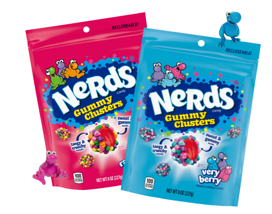
Image of Nerds Gummy Clusters from nerdscandy.com

Firms differ on the extent to which they rely on market research—such as focus groups or polls of consumers—when introducing a new product or overhauling an existing product. Henry Ford became the richest man in the United States by introducing the Model T, the first low-priced and reliable mass-produced automobile. But Ford once remarked that if before introducing the Model T he had asked people the best way to improve transportation they would probably have told him to develop a faster horse. (Note that there’s a debate as to whether Ford ever actually made this observation.) Apple co-founder Steve Jobs took a similar view, once remaking in an interview that “it’s really hard to design products by focus groups. A lot of times, people don’t know what they want until you show it to them.” In another interview, Jobs stated: “We do no market research. We don’t hire consultants.”

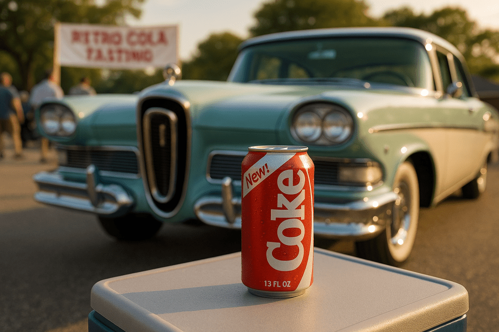
Unsurprisingly, not all new products large firms introduce are successful—whether the products were developed as a result of market research or relied on the hunches of a company’s managers. To take two famous examples, consider the products shown in image at the beginning of this post—“New Coke” and the Ford Edsel.

Pepsi and Coke have been in an intense rivalry for decades. In the 1980s, Pepsi began to gain market share at Coke’s expense as a result of television commercials showcasing the “Pepsi Challenge.” The Pepsi Challenge had consumers choose from colas in two unlabeled cups. Consumers overwhelming chose the cup containing Pepsi. Coke’s management came to believe that Pepsi was winning the blind taste tests because Pepsi was sweeter than Coke and consumers tend to favor sweeter colas. In 1985, Coke’s managers decided to replace the existing Coke formula—which had been largely unchanged for almost 100 years—with New Coke, which had a sweeter taste. Unfortunately for Coke’s managers, consumers’ reaction to New Coke was strongly negative. Less than three months later, the company reintroduced the original Coke, now labeled “Coke Classic.” Although Coke produced both versions of the cola for a number of years, eventually they stopped selling New Coke.

Through the 1920s, the Ford Motor Company produced only two car models—the low-priced Model T and the high-priced Lincoln. That strategy left an opening for General Motors during the 1920s to introduce a variety of car models at a number of price levels. Ford scrambled during the 1930s and after the end of World War II in 1945 to add new models that would compete directly with some of GM’s models. After a major investment in new capacity and an elaborate marketing campaign, Ford introduced the Edsel in September 1957 to compete against GM’s mid-priced models: Pontiac, Oldsmobile, and Buick.

Unfortunately, the Edsel was introduced during a sharp, although relatively short, economic recession. As we discuss in Macroeconomics, Chapter 13 (Economics, Chapter 23), consumers typically cut back on purchases of consumer durables like automobiles during a recession. In addition, the Edsel suffered from reliability problems and many consumers disliked the unusual design, particularly of the front of the car. Consumers were also puzzled by the name Edsel. Ford CEO Henry Ford II was the grandson of Henry Ford and the son of Edsel Ford, who had died in 1943. Henry Ford II named in the car in honor of his father but the unusual name didn’t appeal to consumers. Ford ceased production of the car in November 1959 after losing $250 million, which was one of the largest losses in business history to that point. The name “Edsel” has lived on as a synonym for a disastrous product launch.

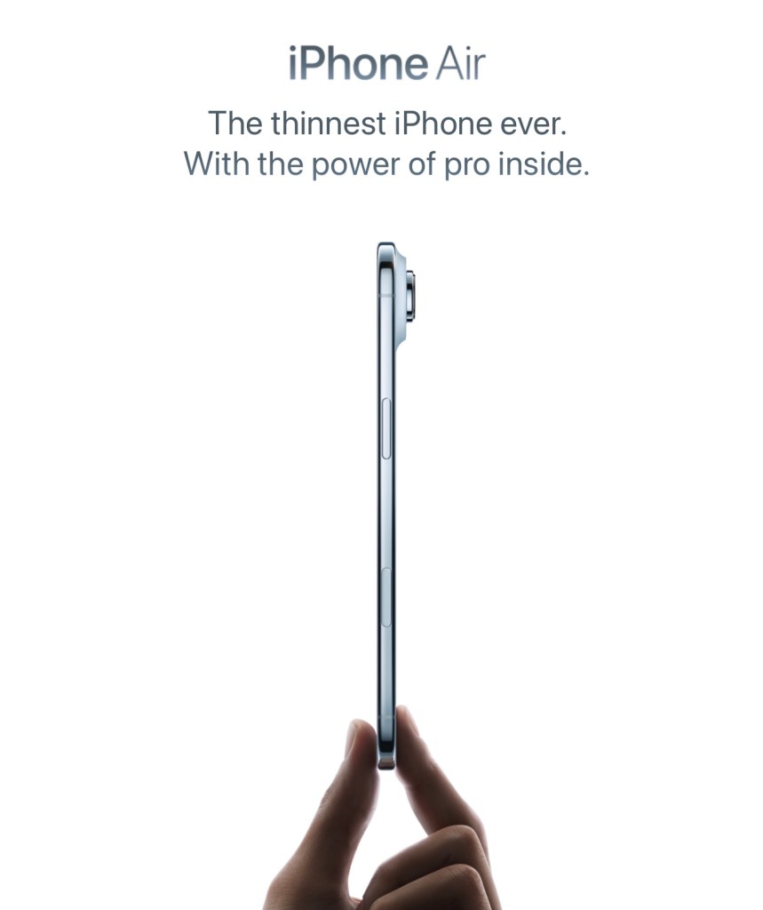
Image of iPhone Air from apple.com

Apple earns about half of its revenue and more than half of its profit from iPhone sales. Making sure that it is able to match or exceed the smartphone features offered by competitors is a top priority for CEO Tim Cook and other Apple managers. Because Apple’s iPhones are higher-priced than many other smartphones, Apple has tried various approaches to competing in the market for lower-priced smartphones.

In 2013, Apple was successful in introducing the iPad Air, a thinner, lower-priced version of its popular iPad. Apple introduced the iPhone Air in September 2025, hoping to duplicate the success of the iPad Air. The iPhone Air has a titanium frame and is lighter than the regular iPhone model. The Air is also thinner, which means that its camera, speaker, and its battery are all a step down from the regular iPhone 17 model. In addition, while the iPhone Air’s price is $100 lower than the iPhone 17 Pro, it’s $200 higher than the base model iPhone 17.

Unlike with the iPad Air, Apple doesn’t seem to have aimed the iPhone Air at consumers looking for a lower-priced alternative. Instead, Apple appears to have targeted consumers who value a thinner, lighter phone that appears more stylish, because of its titanium frame, and who are willing to sacrifice some camera and sound quality, as well as battery life. An article in the Wall Street Journal declared that: “The Air is the company’s most innovative smartphone design since the iPhone X in 2017.” As it has turned out, there are apparently fewer consumers who value this mix of features in a smartphone than Apple had expected.

Sales were sufficiently disappointing that within a month of its introduction, Apple ordered suppliers to cut back production of iPhone Air components by more than 80 percent. Apple was expected to produce 1 million fewer iPhone Airs during 2025 than the company had initially planned. An article in the Wall Street Journal labeled the iPhone Air “a marketing win and a sales flop.” According to a survey by the KeyBanc investment firm there was “virtually no demand for [the] iPhone Air.”

Was Apple having its New Coke moment? There seems little doubt that the iPhone Air has been a very disappointing new product launch. But its very slow sales haven’t inflicted nearly the damage that New Coke caused Coca-Cola or that the Edsel caused Ford. A particularly damaging aspect of New Coke was that was meant as a replacement for the existing Coke, which was being pulled from production. The result was a larger decline in sales than if New Coke had been offered for sale alongside the existing Coke. Similarly, Ford set up a whole new division of the company to produce and sell the Edsel. When Edsel production had to be stopped after only two years, the losses were much greater than they would have been if Edsel production hadn’t been planned to be such a large fraction of Ford’s total production of automobiles.

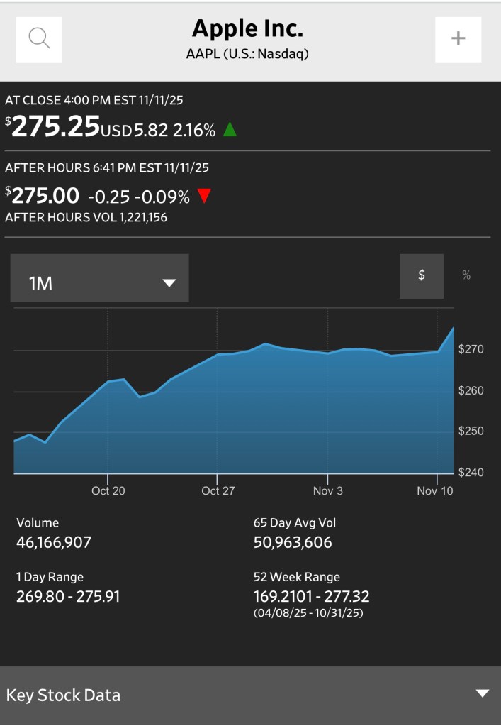
Although very slow iPhone Air sales have caused Apple to incur losses on the model, the Air was meant to be one of several iPhone models and not the only iPhone model. Clearly investors don’t believe that problems with the Air will matter much to Apple’s profits in the long run. The following graphic from the Wall Street Journal shows that Apple’s stock price has kept rising even after news of serious problems with Air sales became public in late October.

So, while the iPhone Air will likely go down as a failed product launch, it won’t achieve the legendary status of New Coke or the Edsel.

Solved Problem: The Fed’s Dilemma

Supports: Macroeconomics, Chapter 13, Section 13.3; Economics, Chapter 23, Section 23.3; and Essentials of Economics, Chapter 15, Section 15.3

Image generated by ChatGPT

A recent article on axios.com made the following observation: “The mainstream view on the Federal Open Market Committee is based on risk management—that the possibility of a further downshift in the job market appears to be the more pressing concern than the chance that inflation will spiral higher.” The article also notes that: “Tariffs’ effects on inflation are probably a one-time bump.”

a. What is the dual mandate that Congress has given the Federal Reserve?

b. In what circumstances might the Federal Open Market Committee (FOMC) be faced with a conflict between the goals in the dual mandate?

c. What does the author mean by tariffs’ effects on inflation being a “one-time bump”?

d. What does the author mean by the FOMC engaging in “risk management”? What is a “downshift” in the labor market? If the FOMC is more concerned about a downshift in the labor market than about inflation, will the committee raise or lower its target for the federal funds rate? Briefly explain.

Solving the Problem
Step 1: Review the chapter material. This problem is about the policy dilemma the Fed can face when the unemployment rate and the inflation rate are both rising, so you may want to review Macroeconomics, Chapter 13, Section 13.3, “Macroeconomic Equilibrium in the Long Run and the Short Run.”

Step 2: Answer part a. by explaining what the Fed’s dual mandate is. Congress has given the Fed a dual mandate of achieving price stability and maximum employment.

Step 3: Answer part b. by explaining when the FOMC may face a conflict with respect to its dual mandate. When the FOMC is faced with rising unemployment and falling inflation, its preferred policy response is clear: The committee will lower its target for the federal funds rate in order to increase the growth of aggregate demand, which will increase real GDP and reduce unemployment. When the FOMC is faced with falling unemployment and rising inflation, its preferred policy response is also clear: The committee will raise its target for the federal funds rate in order to slow the growth of aggregate demand, which will reduce the inflation rate.

But when the Fed faces an aggregate supply shock, its preferred policy response is unclear. An aggregate supply shock, such as the U.S. economy experienced during the Covid pandemic and again with the tariff increases that the Trump administration began implementing in April, will shift the short-run aggregate supply curve (SRAS) will shift to the left, causing an increase in the price level, along with a decline in real GDP and employment. This combination of rising unemployment and inflation is called stagflation. In this situation, the FOMC faces a policy dilemma: Raising the target for the federal funds rate will help reduce inflation, but will likely increase unemployment, while lowering the target for the federal funds rate will lead to lower unemployment, but will likely increase inflation. The following figure shows the situation during the Covid pandemic when the economy experienced both an aggregate demand and aggregate supply shock. The aggregate demand curve and the aggregate supply curve both shifted to the left, resulting in falling real GDP (and employment) and a rising price level.

Step 4: Answer part c. by explaining what it means to refer to the effect of tariffs on inflation being a “one-time bump.” Tariffs cause the aggregate supply curve to shift to the left because by increasing the prices of raw materials and other inputs, they increase the production costs of some businesses. Assuming that tariffs are not continually increasing, their effect on the price level will end once the production costs of firms stop rising.

Step 5: Answer part d. by explaining what the author means by the FOMC engaing in “risk management,” explaining what a “downshift” in the labor is, and whether if the FOMC is more concerned about a downshift in the labor market than in inflation, it will raise or lower its target for the federal funds rate. The article refers to the “possibility” of a further downshift in the labor market. A downshift in the labor market means that the demand for labor may decline, raising the unemployment rate. Managing the risk of this possibility would involve concentrating on the maximum employment part of the Fed’s dual mandate by lowering its target for the federal funds rate. Note that the expectation that the effect of tariffs on the price level is a one-time bump makes it easier for the committee to focus on the maximum employment part of its mandate because the increase in inflation due to the tariff increases won’t persist.

Labor Market Remains Strong

Image generated by ChatGTP 4o

This morning (June 6), the Bureau of Labor Statistics (BLS) released its “Employment Situation” report (often called the “jobs report”) for May. The data in the report show that the labor market continues to be strong. There have been many stories in the media about businesspeople becoming pessimistic as a result of the large tariff increases the Trump Administration announced on April 2—some of which have since been reduced—but we don’t see the effects in the employment data. Some firms may be maintaining employment until they receive greater clarity about where tariff rates will end up. Similarly, although there are some indications that consumer spending may be slowing, to this point, the effects are not evident in the labor market.

The jobs report has two estimates of the change in employment during the month: one estimate from the establishment survey, often referred to as the payroll survey, and one from the household survey. As we discuss in Macroeconomics, Chapter 9, Section 9.1 (Economics, Chapter 19, Section 19.1), many economists and Federal Reserve policymakers believe that employment data from the establishment survey provide a more accurate indicator of the state of the labor market than do the household survey’s employment data and unemployment data. (The groups included in the employment estimates from the two surveys are somewhat different, as we discuss in this post.)

According to the establishment survey, there was a net increase of 139,000 nonfarm jobs during May. This increase was above the increase of 125,000 that economists surveyed had forecast. Somewhat offsetting this increase, the BLS revised downward its previous estimates of employment in March and April by a combined 95,000 jobs. (The BLS notes that: “Monthly revisions result from additional reports received from businesses and government agencies since the last published estimates and from the recalculation of seasonal factors.”) The following figure from the jobs report shows the net change in nonfarm payroll employment for each month in the last two years.

The unemployment rate was unchanged to 4.2 percent in May. As the following figure shows, the unemployment rate has been remarkably stable over the past year, staying between 4.0 percent and 4.2 percent in each month since May 2024. In March, the members of the Federal Open Market Committee (FOMC) forecast that the unemployment rate for 2025 would average 4.4 percent.

As the following figure shows, the monthly net change in jobs from the household survey moves much more erratically than does the net change in jobs from the establishment survey. As measured by the household survey, there was a net decrease of 696,000 jobs in May, following an increase of 461,000 jobs in April. As an indication of the volatility in the employment changes in the household survey note the very large swings in net new jobs in January and February. In any particular month, the story told by the two surveys can be inconsistent with employment increasing in one survey while falling in the other. This month, the discrepancy between the two surveys in their estimates of the change in net jobs was particularly large. (In this blog post, we discuss the differences between the employment estimates in the two surveys.)

The household survey has another important labor market indicator. The employment-population ratio for prime age workers—those aged 25 to 54—declined from 80.7 percent in April to 80.5 percent in May. The prime-age employment-population ratio is somewhat below the high of 80.9 percent in mid-2024, but is above what the ratio was in any month during the period from January 2008 to December 2019.

It remains unclear how many federal workers have been laid off since the Trump Administration took office. The establishment survey shows a decline in total federal government employment of 22,000 in May and a total decline of 59,000 beginning in February. However, the BLS notes that: “Employees on paid leave or receiving ongoing severance pay are counted as employed in the establishment survey.” It’s possible that as more federal employees end their period of receiving severance pay, future jobs reports may report a larger decline in federal employment. To this point, the decline in federal employment has been too small to have a significant effect on the overall labor market.

The establishment survey also includes data on average hourly earnings (AHE). As we noted in this post, many economists and policymakers believe the employment cost index (ECI) is a better measure of wage pressures in the economy than is the AHE. The AHE does have the important advantage of being available monthly, whereas the ECI is only available quarterly. The following figure shows the percentage change in the AHE from the same month in the previous year. The AHE increased 3.9 percent in May. Movements in AHE have been remarkably stable, showing increases of 3.9 percent each month since January.

The following figure shows wage inflation calculated by compounding the current month’s rate over an entire year. (The figure above shows what is sometimes called 12-month wage inflation, whereas this figure shows 1-month wage inflation.) One-month wage inflation is much more volatile than 12-month wage inflation—note the very large swings in 1-month wage inflation in April and May 2020 during the business closures caused by the Covid pandemic. In May, the 1-month rate of wage inflation was 5.1 percent, up sharply from 2.4 percent in April. If the 1-month increase in AHE is sustained, it would indicate that the Fed will struggle to achieve its 2 percent target rate of price inflation. But one month’s data from such a volatile series may not accurately reflect longer-run trends in wage inflation.

Today’s jobs report leaves the situation facing the Federal Reserve’s policy-making Federal Open Market Committee (FOMC) largely unchanged. Looming over monetary policy, however, is the expected effect of the Trump Administration’s tariff increases. As we note in this blog post, a large unexpected increase in tariffs results in an aggregate supply shock to the economy. In terms of the basic aggregate demand and aggregate supply model that we discuss in Macroeconomics, Chapter 13 (Economics, Chapter 23), an unexpected increase in tariffs shifts the short-run aggregate supply curve (SRAS) to the left, increasing the price level and reducing the level of real GDP.

One indication of expectations of future changes in the FOMC’s target for the federal funds rate comes from investors who buy and sell federal funds futures contracts. (We discuss the futures market for federal funds in this blog post.) The data from the futures market indicate that, despite the potential effects of the tariff increases, investors don’t expect that the FOMC will cut its target for the federal funds rate at its June 17–18 meeting. As shown in the following figure, investors assign a 99.9 percent probability to the committee keeping its target unchanged at 4.25 percent to 4.50 percent at that meeting.

As the following figure shows, investors don’t expect the FOMC to cut its federal funds rate target until the committee’s September 16-17 meeting. Investors assign a probability of 54.6 percent that at that meeting the committee will cut its target range by 0.25 percentage point (25 basis points) to 4.00 percent to 4.25 percent. And a probability of 9.4 percent that the committee will cut its target rate by 50 baisis points to 3.75 percent to 4.00 percent. At 35.9 percent, investors assign a fairly high probability to the committee keeping its target range constant at that meeting.

A Disagreement between Fed Chair Powell and Fed Governor Waller over Monetary Policy, and Can President Trump Replace Powell?

In this photo of a Federal Open Market Committee meeting, Fed Chair Jerome Powell is on the far left and Fed Governor Christopher Waller is the third person to Powell’s left. (Photo from federalreserve.gov)

This post discusses two developments this week that involve the Federal Reserve. First, we discuss the apparent disagreement between Fed Chair Jerome Powell and Fed Governor Christopher Waller over the best way to respond to the Trump Administration’s tariff increases. As we discuss in this blog post and in this podcast, in terms of the aggregate demand and aggregate supply model, a large unexpected increase in tariffs results in an aggregate supply shock to the economy, shifting the short-run aggregate supply curve (SRAS) to the left. The following is Figure 13.7 from Macroeconomics (Figure 23.7 from Economics) and illustrates the effects of an aggregate supply shock on short-run macroeconomic equilibrium.

Although the figure shows the effects of an aggregate supply shock that results from an unexpected increase in oil prices, using this model, the result is the same for an aggregate supply shock caused by an unexpected increase in tariffs. Two-thirds of U.S. imports are raw materials, intermediate goods, or capital goods, all of which are used as inputs by U.S. firms. So, in both the case of an increase in oil prices and in the case of an increase in tariffs, the result of the supply shock is an increase in U.S. firms’ production costs. This increase in costs reduces the quantity of goods firms will supply at every price level, shifting the SRAS curve to the left, as shown in panel (a) of the figure. In the new macroeconomic equilibrium, point B in panel (a), the price level increases and the level of real GDP declines. The decline in real GDP will likely result in an increase in the unemployment rate.

An aggregate supply shock poses a policy dilemma for the Fed’s policymaking Federal Open Market Committee (FOMC). If the FOMC responds to the decline n real GDP and the increase in the unemployment rate with an expansionary monetary policy of lowering the target for the federal funds rate, the result is likely to be a further increase in the price level. Using a contractionary monetary policy of increasing the target for the federla funds rate to deal with the rising price level can cause real GDP to fall further, possibly pushing the economy into a recession. One way to avoid the policy dilemma from an aggregate supply shock caused by an increase in tariffs is for the FOMC to “look through”—that is, not respond—to the increase in tariffs. As panel (b) in the figure shows, if the FOMC looks through the tariff increase, the effect of the aggregate supply shock can be transitory as the economy absorbs the one-time increase in the price level. In time, real GDP will return to equilibrium at potential real GDP and the unemployment rate will fall back to the natural rate of unemployment.

On Monday (April 14), Fed Governor Christopher Waller in a speech to the Certified Financial Analysts Society of St. Louis made the argument for either looking through the macroeconomic effects of the tariff increase—even if the tariff increase turns out to be large, which at this time is unclear—or responding to the negative effects of the tariffs increases on real GDP and unemployment:

“I am saying that I expect that elevated inflation would be temporary, and ‘temporary’ is another word for ‘transitory.’ Despite the fact that the last surge of inflation beginning in 2021 lasted longer than I and other policymakers initially expected, my best judgment is that higher inflation from tariffs will be temporary…. While I expect the inflationary effects of higher tariffs to be temporary, their effects on output and employment could be longer-lasting and an important factor in determining the appropriate stance of monetary policy. If the slowdown is significant and even threatens a recession, then I would expect to favor cutting the FOMC’s policy rate sooner, and to a greater extent than I had previously thought.”

In a press conference after the last FOMC meeting on March 19, Fed Chair Jerome Powell took a similar position, arguing that: “If there’s an inflation that’s going to go away on its own, it’s not the correct response to tighten policy.” But in a speech yesterday (April 16) at the Economic Club of Chicago, Powell indicated that looking through the increase in the price level resulting from a tariff increase might be a mistake:

“The level of the tariff increases announced so far is significantly larger than anticipated. The same is likely to be true of the economic effects, which will include higher inflation and slower growth. Both survey- and market-based measures of near-term inflation expectations have moved up significantly, with survey participants pointing to tariffs…. Tariffs are highly likely to generate at least a temporary rise in inflation. The inflationary effects could also be more persistent…. Our obligation is to keep longer-term inflation expectations well anchored and to make certain that a one-time increase in the price level does not become an ongoing inflation problem.”

In a discussion following his speech, Powell argued that tariff increases may disrupt global supply chains for some U.S. industries, such as automobiles, in way that could be similar to the disruptions caused by the Covid pandemic of 2020. As a result: “When you think about supply disruptions, that is the kind of thing that can take time to resolve and it can lead what would’ve been a one-time inflation shock to be extended, perhaps more persistent.” Whereas Waller seemed to indicate that as a result of the tariff increases the FOMC might be led to cut its target for the federal funds sooner or to larger extent in order to meet the maximum employment part of its dual mandate, Powell seemed to indicate that the FOMC might keep its target unchanged longer in order to meet the price stability part of the dual mandate.

Powell’s speech caught the notice of President Donald Trump who has been pushing the FOMC to cut its target for the federal funds rate sooner. An article in the Wall Street Journal, quoted Trump as posting to social media that: “Powell’s termination cannot come fast enough!” Powell’s term as Fed chair is scheduled to end in May 2026. Does Trump have the legal authority to replace Powell earlier than that? As we discuss in Macroeconomics, Chapter 27 (Economics Chapter 17), according to the Federal Reserve Act, once a Fed chair is notimated to a four-year term by the president (President Trump first nominated Powell to be chair in 2017 and Powell took office in 2018) and confirmed by the Senate, the president cannot remove the Fed chair except “for cause.” Most legal scholars argue that a president cannot remove a Fed chair due to a disagreement over monetary policy.

Article I, Section II of the Constitution of the United States states that: “The executive Power shall be vested in a President of the United States of America.” The ability of Congress to limit the president’s power to appoint and remove heads of commissions, agencies, and other bodies in the executive branch of government—such as the Federal Reserve—is not clearly specified in the Constitution. In 1935, a unanimous Supreme Court ruled in the case of Humphrey’s Executor v. United States that President Franklin Roosevelt couldn’t remove a member of the Federal Trade Commission (FTC) because in creating the FTC, Congress specified that members could only be removed for cause. Legal scholars have presumed that the ruling in this case would also bar attempts by a president to remove members of the Fed’s Board of Governors because of a disagreement over monetary policy.

The Trump Administration recently fired a member of the National Labor Relations Board and a member of the Merit Systems Protection Board. The members sued and the Supreme Court is considering the case. The Trump Adminstration is asking the Court to overturn the Humphrey’s Executor decision as having been wrongly decided because the decision infringed on the executive power given to the president by the Constitution. If the Court agrees with the administration and overturns the precdent established by Humphrey’s Executor, would President Trump be free to fire Chair Powell before Powell’s term ends? (An overview of the issues involved in this Court case can be found in this article from the Associated Press.)

The answer isn’t clear because, as we’ve noted in Macroeconomics, Chapter 14, Section 14.4, Congress gave the Fed an unusual hybrid public-private structure and the ability to fund its own operations without needing appropriations from Congress. It’s possible that the Court would rule that in overturning Humphrey’s Executor—if the Court should decide to do that—it wasn’t authorizing the president to replace the Fed chair at will. In response to a question following his speech yesterday, Powell seemed to indicate that the Fed’s unique structure might shield it from the effects of the Court’s decision.

If the Court were to overturn its ruling in Humphrey’s Executor and indicate that the ruling did authorize the president to remove the Fed chair, the Fed’s ability to conduce monetary policy independently of the president would be seriously undermined. In Macroeconomics, Chapter 17, Section 17.4 we review the arguments for and against Fed independence. It’s unclear at this point when the Court might rule on the case.

Surprisingly Strong CPI Report

Photo courtesy of Lena Buonanno.

As we’ve discussed in several blog posts (for instance, here and here), recent macro data have been consistent with the Federal Reserve being close to achieving a soft landing. The Fed’s increases in its target for the federal funds rate have slowed the growth of aggregate demand sufficiently to bring inflation closer to the Fed’s 2 percent target, but haven’t, to this point, slowed the growth of aggregate demand so much that the U.S. economy has been pushed into a recession.

By January 2024, many investors in financial markets and some economists were expecting that at its meeting on March 19-20, the Fed’s Federal Open Market Committee would be cutting its target for the federal funds. However, members of the committee—notably, Chair Jerome Powell—have been cautious about assuming prematurely that inflation had, in fact, been brought under control. In fact, in his press conference on January 31, following the committee’s most recent meeting, Powell made clear that the committee was unlikely to reduce its target for the federal funds rate at its March meeting. Powell noted that “inflation is still too high, ongoing progress in bringing it down is not assured, and the path forward is uncertain.”

Powell’s caution seemed justified when, on February 2, the Bureau of Labor Statistics (BLS) released its most recent “Employment Situation Report” (discussed in this post). The report’s data on growth in employment and growth in wages, as measured by the change in average hourly earnings, might be indicating that aggregate demand is growing too rapidly for inflation to continue to decline.

The BLS’s release today (February 13) of its report on the consumer price index (CPI) (found here) for January provided additional evidence that the Fed may not yet have put inflation on a firm path back to its 2 percent target. The average forecast of economists surveyed before the release of the report was that the increase in the version of the CPI that includes the prices of all goods and services in the market basket—often called headline inflation—would be 2.9 percent. (We discuss how the BLS constructs the CPI in Macroeconomics, Chapter 9, Section 19.4, Economics, Chapter 19, Section 19.4, and Essentials of Economics, Chapter 3, Section 13.4.) As the following figure shows, headline inflation for January was higher than expected at 3.1 percent (measured by the percentage change from the same month in the previous year), while core inflation—which excludes the prices of food and energy—was 3.9 percent. Headline inflation was lower than in December 2023, while core inflation was almost unchanged.

Although the values for January might seem consistent with a gradual decline in inflation, that conclusion may be misleading. Headline inflation in January 2023 had been surprisingly high at 6.4 percent. Hence, the comparision between the value of the CPI in January 2024 with the value in January 2023 may be making the annual CPI inflation rate seem artificially low. If we look at the 1-month inflation rate for headline and core inflation—that is the annual inflation rate calculated by compounding the current month’s rate over an entire year—the values are more concerning, as indicated in the following figure. Headline CPI inflation is 3.7 percent and core CPI inflation is 4.8 percent.

Even more concerning is the path of inflation in the prices of services. Chair Powell has emphasized that as supply chain problems have gradually been resolved, inflation in the prices of goods has been rapidly declining. But inflaion in services hasn’t declined nearly as much. Last summer he stated the point this way:

“Part of the reason for the modest decline of nonhousing services inflation so far is that many of these services were less affected by global supply chain bottlenecks and are generally thought to be less interest sensitive than other sectors such as housing or durable goods. Production of these services is also relatively labor intensive, and the labor market remains tight. Given the size of this sector, some further progress here will be essential to restoring price stability.”

The following figure shows the 1-month inflation rate in services prices. The figure shows that inflation in services has been above 4 percent in every month since July 2023. Inflation in services was a very high 8.7 percent in January. Clearly such large increases in the prices of services aren’t consistent with the Fed meeting its 2 percent inflation target.

How should we interpret the latest CPI report? First, it’s worth bearing in mind that a single month’s report shouldn’t be relied on too heavily. There can be a lot of volatility in the data month-to-month. For instance, inflation in the prices of services jumped from 4.7 percent in December to 8.7 percent in January. It seems unlikely that inflation in the prices of services will continue to be over 8 percent.

Second, housing prices are a large component of service prices and housing prices can be difficult to measure accurately. Notably, the BLS includes in its measure the implicit rental price that someone who owns his or her own home pays. The BLS calculates that implict rental price by asking consumers who own their own homes the following question: “If someone were to rent your home today, how much do you think it would rent for monthly, unfurnished and without utilities?” (The BLS discusses how it measures the price of housing services here.) In practice, it may be difficult for consumers to accurately answer the question if very few houses similar to theirs are currently for rent in their neighborhood.

Third, the Fed uses the personal consumption expenditures (PCE) price index, not the CPI, to gauge whether it is achieving its 2 percent inflation target. The Bureau of Economic Analysis (BEA) includes the prices of more goods and services in the PCE than the BLS includes in the CPI and measures housing services using a different approach than that used by the BLS. Although inflation as measured by changes in the CPI and as measured by changes in the PCE move roughly together over long periods, the two measures can differ significantly over a period of a few months. The difference between the two inflation measures is another reason not to rely too heavily on a single month’s CPI data.

Despite these points, investors on Wall Street clearly interpreted the CPI report as bad news. Investors have been expecting that the Fed will soon cut its target for the federal funds rate, which should lead to declines in other key interest rates. If inflation continues to run well above the Fed’s 2 percent target, it seems likely that the Fed will keep its federal funds target at its current level for longer, thereby slowing the growth of aggregate demand and raising the risk of a recession later this year. Accordingly, the Dow Jones Industrial Average declined by more than 500 points today (February 13) and the interest rate on the 10-year Treasury note rose above 4.3 percent.

The FOMC has more than a month before its next meeting to consider the implications of the latest CPI report and the additional macro data that will be released in the meantime.

The Return of the FedEx Indicator?

On September 16, 2022 an article in the Wall Street Journal had the headline: “Economic Worries, Weak FedEx Results Push Stocks Lower.” Another article in the Wall Street Journal noted that: “The company’s downbeat forecasts, announced Thursday, intensified investors’ macroeconomic worries.”

Why would the news that FedEx had lower revenues than expected during the preceding weeks cause a decline in stock market indexes like the Dow Jones Industrial Average and the S&P 500? As the article explained: “Delivery companies [such as FedEx and its rival UPS) are the proverbial canary in the coal mine for the economy.” In other words, investors were using FedEx’s decline in revenue as a leading indicator of the business cycle. A leading indicator is an economic data series—in this case FedEx’s revenue—that starts to decline before real GDP and employment in the months before a recession and starts to increase before real GDP and employment in the months before a recession reaches a trough and turns into an expansion.

So, investors were afraid that FedEx’s falling revenue was a signal that the U.S. economy would soon enter a recession. And, in fact, FedEx CEO Raj Subramaniam was quoted as believing that the global economy would fall into a recession. As firms’ profits decline during a recession so, typically, do the prices of the firms’ stock. (As we discuss in Macroeconomics, Chapter 6, Section 6.2 and in Economics, Chapter 8, Section 8.2, stock prices reflect investors’ expectations of the future profitability of the firms issuing the stock.)

Monitoring fluctuations in FedEx’s revenue for indications of the future course of the economy is nothing new. When Alan Greenspan was chair of the Federal Reserve from 1987 to 2006, he spoke regularly with Fred Smith, the founder of FedEx and at the time CEO of the firm. Greenspan believed that changes in the number of packages FedEx shipped gave a good indication of the overall state of the economy. FedEx plays such a large role in moving packages around the country that most economists agree that there is a close relationship between fluctuations in FedEx’s business and fluctuations in GDP. Some Wall Street analysts refer to this relationship as the “FedEx Indicator” of how the economy is doing.

In September 2022, the FedEx indicator was blinking red. But the U.S. economy is complex and fluctuations in any indicator can sometimes provide an inaccurate forecast of when a recession will begin or end. And, in fact, some investment analysts believed that problems at FedEx may have been due as much to mistakes the firms’ managers had made as to general problems in the economy. As one analyst put it: “We believe a meaningful portion of FedEx’s missteps here are company-specific.”

At this point, Fed Chair Jerome Powell and the other members of the Federal Open Market Committee are still hoping that they can bring the economy in for a soft landing—bringing inflation down closer to the Fed’s 2 percent target, without bringing on a recession—despite some signals, like those being given by the FedEx indicator, that the probability of the United States entering a recession was increasing.

Sources: Will Feuer, “FedEx Stock Tumbles More Than 20% After Warning on Economic Trends,” Wall Street Journal, September 16, 2022; Alex Frangos and Hannah Miao, “ FedExt Stock Hit by Profit Warning; Rivals Also Drop Amid Recession Fears,” Wall Street Journal, September 16, 2022; Richard Clough, “FedEx has Biggest Drop in Over 40 Years After Pulling Forecast,” bloomberg.com, September 16, 2022; and David Gaffen, “The FedEx Indicator,” Wall Street Journal, February 20, 2007.

Senator Elizabeth Warren vs. Economist Lawrence Summers on Monetary Policy

Senator Elizabeth Warren (Photo from the Associated Press)

Lawrence Summers (Photo from harvardmagazine.com)

As we’ve discussed in several previous blog posts, in early 2021 Lawrence Summers, professor of economics at Harvard and secretary of the treasury in the Clinton administration, argued that the Biden administration’s $1.9 trillion American Rescue Plan, enacted in March, was likely to cause a sharp acceleration in inflation. When inflation began to rapidly increase, Summers urged the Federal Reserve to raise its target for the federal funds rate in order to slow the increase in aggregate demand, but the Fed was slow to do so. Some members of the Federal Open Market Committee (FOMC) argued that much of the inflation during 2021 was transitory in that it had been caused by lingering supply chain problems initially caused by the Covid–19 pandemic.

At the beginning of 2022, most members of the FOMC became convinced that in fact increases in aggregate demand were playing an important role in causing high inflation rates. Accordingly, the FOMC began increasing its target for the federal funds rate in March 2022. After two more rate increases, on the eve of the FOMC’s meeting on July 26–27, the federal funds rate target was a range of 1.50 percent to 1.75 percent. The FOMC was expected to raise its target by at least 0.75 percent at the meeting. The following figure shows movements in the effective federal funds rate—which can differ somewhat from the target rate—from January 1, 2015 to July 21, 2022.

In an opinion column in the Wall Street Journal, Massachusetts Senator Elizabeth Warren argued that the FOMC was making a mistake by increasing its target for the federal funds rate. She also criticized Summers for supporting the increases. Warren worried that the rate increases were likely to cause a recession and argued that Congress and President Biden should adopt alternative measures to contain inflation. Warren argued that a better approach to dealing with inflation would be to, among other steps, increase the federal government’s support for child care to enable more parents to work, provide support for strengthening supply chains, and lower prescription drug prices by allowing Medicare to negotiate the prices with pharmaceutical firms. She also urged a “crack down on price gouging by large corporations.” (We discussed the argument that monopoly power is responsible for inflation in this blog post.)

Summers responded to Warren in a Twitter thread. He noted that: “In the 18 months since the massive stimulus policies & easy money that [Senator Warren] has favored & I have opposed, the inflation rate has risen from below 2 to above 9 percent & workers purchasing power has, as a consequence, declined more rapidly than in any year in the last 50.” And “[Senator Warren] opposes restrictive monetary policy or any other measure to cool off total demand. Why does she think at a time when there are twice as many vacancies as jobs that inflation will come down without some drop in total demand?”

Clearly, economists and policymakers continue to hotly debate monetary policy.

Source: Elizabeth Warren, “Jerome Powell’s Fed Pursues a Painful and Ineffective Inflation Cure,” Wall Street Journal, July 24, 2022.

Was the High Inflation of 2021–2022 Due to Shifts in Aggregate Demand or Shifts in Aggregate Supply?

Man surprised by inflation in food prices.

To answer the question in the title: Negative supply shocks—shifts to the left in the short-run aggregate supply (SRSAS) curve—and positive demand shocks—shifts to the right in the aggregate demand (AD) curve—both contributed to the acceleration in inflation that began in the spring of 2021. But were the aggregate supply shifts, such as the semiconductor shortage that reduced the supply of new automobiles, more or less important than the aggregate demand shifts, such as the expansionary monetary and fiscal policies?

Adam Hale Shapiro of the Federal Reserve Bank of San Francisco used a basic piece of microeconomic analysis to estimate the contribution of shifts in aggregate supply and shifts in aggregate demand to inflation during this period. He looked at the prices of the more than 100 categories of goods and services in the personal consumption expenditures(PCE) price index. The PCE price index is a measure of the price level similar to the GDP deflator, except it includes only the prices of goods and services from the consumption category of GDP. Changes in the PCE price index are the Federal Reserve’s preferred measure of the inflation rate because that index includes the prices of more goods and services than are included in the consumer price index (CPI).

Shapiro explains how he used microeconomic reasoning to determine whether prices in one of the more than 100 categories of goods and services were increasing because of shifts in supply or because of shifts in demand:

“Shifts in demand move both prices and quantities in the same direction along the upward-sloping supply curve, meaning prices rise as demand increases. Shifts in supply move prices and quantities in opposite directions along the downward-sloping demand curve, meaning prices rise when supplies decline.”

For example, the figure on the left shows the effect on the market for toys of an increase in the demand for toys. (We discuss how shifts in demand and supply curves in a market affect equilibrium price and quantity in Chapter 3, Section 3.4 of Economics, Macroeconomics, and Microeconomics.) The demand curve for toys shifts to the right from D₁ to D₂, the equilibrium price increases from P₁ to P₂, and the equilibrium quantity increases from Q₁ to Q₂. The figure on the right shows the effect on the market for toys if the price increase results from a decrease in the supply of toys rather than from an increase in demand. The supply curve shifts to the left from S₁ to S₂, the equilibrium price increases from P₁ to P₂, and the equilibrium quantity decreases from Q₁ to Q₂.

Shapiro used statistical methods to determine the part of a change in price or quantity that was unexpected. He took this approach in order to focus on short-run changes in these markets caused by shifts in demand and supply rather than long-run changes resulting from “factors such as technological improvements, cost-of-living adjustments to wages, or demographic changes like population aging.” In some cases, the quantity or the price in a market were very close to their expected values, so Shapiro labeled the cause of a price increase in this market as “ambiguous.”

Shapiro notes that: “Categories that experience frequent supply-driven price changes include food and household products such as dishes, linens, and household paper items. Categories that experience frequent demand-driven price changes include motor vehicle-related products, used cars, and electricity.”

The following figure shows Shapiro’s results for the period from January 2020 through April 2022. The height of each column gives the inflation rate in the month measured as the percentage change in the PCE price index from the same month in the previous year. For example, in March 2022, the inflation rate was 6.6 percent. The height of the yellow segment is the part of inflation in that month attributable to increases in demand, the height of the green segment is the part of the inflation in that month that is attributable to decreases in supply, and the height of the green segment is the part of the inflation that Shapiro can’t assign to either demand or supply. In March 2022, increased in demand accounted for 2.2 percentage points of the total 6.6 percentage point increase in inflation. Decreases in supply accounted for 3.3 percentage points, and the remaining 1.2 percentage points had an ambiguous cause.

We can conclude that, measured this way, the increase in inflation from the spring of 2021 through the spring of 2022 was due more to negative supply shocks than to positive demand shocks.

Source: Adam Hale Shapiro, “How Much Do Supply and Demand Drive Inflation?” Federal Reserve Bank of San Francisco Economic Letter, 22-15, June 21, 2022.

Macroeconomics or Microeconomics? Is a Lack of Competition in Some Industries Behind the Increase in Inflation?

In January 2022, the Bureau of Labor Statistics (BLS) announced that inflation, measured as the percentage change in the consumer price index (CPI) from December 2020 to December 2021, was 7 percent. That was the highest rate since June 1982, which was near the end of the Great Inflation that lasted from 1968 to 1982. The following figure shows the inflation rate since the beginning of 1948.

What explains the surge in inflation? Most economists believe that it is the result of the interaction of increases in aggregate demand resulting from very expansionary monetary and fiscal policy and disruptions to supply in some industries as a result of the Covid-19 pandemic. (We discuss movements in aggregate demand and aggregate supply during the pandemic in the updated editions of Economics, Chapter 23, Section 23.3 and Macroeconomics, Chapter 13, Section, 13.3.)

But President Joe Biden has suggested that mergers and acquisitions in some industries—he singled out meatpacking—have reduced competition and contributed to recent price increases. Massachusetts Senator Elizabeth Warren has made a broader claim about reduced competition being responsible for the surge in inflation: “Market concentration has allowed giant corporations to hide behind claims of increased costs to fatten their profit margins. [Corporations] are raising prices because they can.” And “Corporations are exploiting the pandemic to gouge consumers with higher prices on everyday essentials, from milk to gasoline.”

Do many economists agree that reduced competition explains inflation? The Booth School of Business at the University of Chicago periodically surveys a panel of more than 40 well-known academic economists for their opinions on significant policy issues. Recently, the panel was asked whether they agreed with these statements:

A significant factor behind today’s higher US inflation is dominant corporations in uncompetitive markets taking advantage of their market power to raise prices in order to increase their profit margins.
Antitrust interventions could successfully reduce US inflation over the next 12 months.
Price controls as deployed in the 1970s could successfully reduce US inflation over the next 12 months.

Large majorities of the panel disagreed with statements 1. and 2.—that is, they don’t believe that a lack of competition explains the surge in inflation or that antitrust actions by the federal government would be likely to reduce inflation in the coming year. A smaller majority disagreed with statement 3., although even some of those who agreed that price controls would reduce inflation stated that they believed price controls were an undesirable policy. For instance, while he agreed with statement 3., Oliver Hart of Harvard noted that: “They could reduce inflation but the consequence would be shortages and rationing.”

One way to characterize the panel’s responses is that they agreed that the recent inflation was primarily a macroeconomic issue—involving movements in aggregate demand and aggregate supply—rather than a microeconomic issue—involving the extent of concentration in individual industries.

The panels responses can be found here.

Sources for Biden and Warren quotes: Greg Ip, “Is Inflation a Microeconomic Problem? That’s What Biden’s Competition Push Is Betting,” Wall Street Journal, January 12, 2022; and Patrick Thomas and Catherine Lucey, “Biden Promotes Plan Aimed at Tackling Meat Prices,” Wall Street Journal, January 3, 2022; and https://twitter.com/SenWarren/status/1464353269610954759?s=20

Solved Problem: The Fed’s Policy Dilemma

Supports: Macroneconomics Chapter 15, Section 15.3; Economics Chapter 25, Section 25.3; and Essentials of Economics Chapter 17, Sections 17.3.

Solved Problem: The Fed’s Policy Dilemma

In the fall of 2021, the inflation rate was at its highest level since 2008. The unemployment rate was above 5 percent, which was much lower than in the spring of 2020, but still well above its level of early 2020 before the Covid-19 pandemic. In testifying before Congress, Fed Chair Jerome Powell stated that he believed the high inflation rate was transitory and in the longer run “inflation is expected to drop back toward our longer-run 2 percent goal.”

But Powell also stated that if inflation continued to remain high the Fed would face a policy dilemma. “Almost all of the time, inflation is low when unemployment is high, so interest rates work on both problems.” But in contrast, in the fall of 2021 both the unemployment and inflation rates were high: “That’s the very difficult situation we find ourselves in.”

a. Briefly explain what Powell meant by saying that almost all of the time “interest rates work on both problems.”

b. Why did macroeconomic conditions in the fall of 2021 present Fed policymakers with a “very difficult” situation?

Source: Kate Davidson and Nick Timiraos, “Powell Says Fed Faces ‘Difficult Trade-Off’ if Inflation Doesn’t Moderate,” Wall Street Journal, September 30, 2021; and Chair Jerome H. Powell, “Testimony Before the Committee on Banking, Housing, and Urban Affairs, U.S. Senate, Washington, D.C.” September 28, 2021, federalreserve. gov..

Solving the Problem

Step 1: Review the chapter material. This problem is about the policy situation the Fed faces when the unemployment and inflation rates are both high, so you may want to review Chapter 15, Section 15.3, “Monetary Policy and Economic Activity,” and the discussion of staflation, including Figure 13.7, in Chapter 13, Section 13.3, “Macroeconomic Equilibrium in the Long Run and the Short Run.”

Step 2: Explain what Powell meant by “interest rates work on both problems.” We’ve seen that in the typical recession the unemployment rate increases while the inflation rate decreases. We’ve also seen that if the economy is above potential GDP, the unemployment rate is very low but the inflation rate increases. (To review these facts, see Chapter 10, Section 10.3 “The Business Cycle.”) The Fed uses changes in its target for the federal funds rate to affect the level of real GDP and the price level, as it attempts to hit its policy goals of high employment and price stability.

So “almost all of the time,” the Fed can use interest rates–changes in the target for the federal funds rate–to work on the problems of high unemployment and high inflation–depending on which is occuring during a particular period.

Step 3: Explain why macroeconomic conditions in the fall of 2021 presented Fed policymakers with a “very difficult” situation. As Powell observes, “almost all the time” Fed policy is focused on reducing either high unemployment or high inflation, but not both. As we note in Chapter 13, Section 13.3, economists refer to a situation when the unemployment and inflations rates are both high at the same time as a period of stagflation. If the inflation rate is high, then expansionary monetary policy–a low target for the federal funds rate–will reduce the unemployment rate but make an already high inflation rate even higher. Similarly, if the unemployment rate is high, then contractionary monetary policy–a high target for the federal funds rate–will reduce the inflation rate but make an already high unemploument rate even higher. A very difficult policy dilemma for the Fed!

How did Fed policymakers expect to resolve this difficulty? In his testimony, Powell explained that he believed that the high inflation rate the U.S. economy was experiencing during the fall of 2021 was transitory and would begin to decline once the supply problems caused by the Covid-19 pandemic were resolved in the coming months. Referring to the supply problems he noted that “These aren’t things that we [the Fed] can control.” Therefore, the Fed did not intend to use policy to address the high inflation rate and could continue to pursue an expansionary monetary policy to push the labor market back to full employment.