Authors Glenn Hubbard and Tony O’Brien reconsider the role of inflation in today’s economy. They discuss the Fed’s possible responses by considering responses to similar inflation threats in previous generations – notably the Fed’s response led by Paul Volcker that directly led to the early 1980’s recession. The markets are reflecting stark differences in our collective expectations about what will happen next. Listen to find out more about the Fed’s likely next steps.
Category: Ch19: Unemployment and Inflation
Did the Fed Make a Mistake by Not Preempting Inflation?
Warning: Long post!
It now seems clear that the new monetary policy strategy the Fed announced in August 2020 was a decisive break with the past in one respect: With the new strategy, the Fed abandoned the approach dating to the 1980s of preempting inflation. That is, the Fed would no longer begin raising its target for the federal funds rate when data on unemployment and real GDP growth indicated that inflation was likely to rise. Instead, the Fed would wait until inflation had already risen above its target inflation rate.
Since 2012, the Fed has had an explicit inflation target of 2 percent. As we discussed in a previous blog post, with the new monetary policy the Fed announced in August 2020, the Fed modified how it interpreted its inflation target: “[T]he Committee seeks to achieve inflation that averages 2 percent over time, and therefore judges that, following periods when inflation has been running persistently below 2 percent, appropriate monetary policy will likely aim to achieve inflation moderately above 2 percent for some time.”
The Fed’s new approach is sometimes referred to as average inflation targeting (AIT) because the Fed attempts to achieve its 2 percent target on average over a period of time. But as former Fed Vice Chair Richard Clarida discussed in a speech in November 2020, the Fed’s monetary policy strategy might be better called a flexible average inflation target (FAIT) approach rather than a strictly AIT approach. Clarida noted that the framework was asymmetric, meaning that inflation rates higher than 2 percent need not be offset with inflation rates lower than 2 percent: “The new framework is asymmetric. …[T]he goal of monetary policy … is to return inflation to its 2 percent longer-run goal, but not to push inflation below 2 percent.” And: “Our framework aims … for inflation to average 2 percent over time, but it does not make a … commitment to achieve … inflation outcomes that average 2 percent under any and all circumstances ….”
Inflation began to increase rapidly in mid-2021. The following figure shows three measure of inflation, each calculated as the percentage change in the series from the same month in the previous year: the consumer price index (CPI), the personal consumption expenditure (PCE) price index, and the core PCE—which excludes the prices of food and energy. Inflation as measured by the CPI is sometimes called headline inflation because it’s the measure of inflation that most often appears in media stories about the economy. The PCE is a broader measure of the price level in that it includes the prices of more consumer goods and services than does the CPI. The Fed’s target for the inflation rate is stated in terms of the PCE. Because prices of food and inflation fluctuate more than do the prices of other goods and services, members of the Fed’s Federal Open Market Committee (FOMC) generally consider changes in the core PCE to be the best measure of the underlying rate of inflation.

The figure shows that for most of the period from 2002 through early 2021, inflation as measured by the PCE was below the Fed’s 2 percent target. Since that time, inflation has been running well above the Fed’s target. In February 2022, PCE inflation was 6.4 percent. (Core PCE inflation was 5.4 percent and CPI inflation was 7.9 percent.) At its March 2022 meeting the FOMC begin raising its target for the federal funds rate—well after the increase in inflation had begun. The Fed increased its target for the federal funds rate by 0.25 percent, which raised the target from 0 to 0.25 percent to 0.25 to 0.50 percent.
Should the Fed have taken action to reduce inflation earlier? To answer that question, it’s first worth briefly reviewing Fed policy during the Great Inflation of 1968 to 1982. In the late 1960s, total federal spending grew rapidly as a result of the Great Society social programs and the war in Vietnam. At the same time, the Fed increased the rate of growth of the money supply. The result was an end to the price stability of the 1952-1967 period during which the annual inflation rate had averaged only 1.6 percent.
The 1973 and 1979 oil price shocks also contributed to accelerating inflation. Between January 1974 and June 1982, the annual inflation rate averaged 9.3 percent. This was the first episode of sustained inflation outside of wartime in U.S. history—until now. Although the oil price shocks and expansionary fiscal policy contributed to the Great Inflation, most economists, inside and outside of the Fed, eventually concluded that Fed policy failures were primarily responsible for inflation becoming so severe.
The key errors are usually attributed to Arthur Burns, who was Fed Chair from January 1970 to March 1978. Burns, who was 66 at the time of his appointment, had made his reputation for his work on business cycles, mostly conducted prior to World War II at the National Bureau of Economic Research. Burns was skeptical that monetary policy could have much effect on inflation. He was convinced that inflation was mainly the result of structural factors such as the power of unions to push up wages or the pricing power of large firms in concentrated industries.
Accordingly, Burns was reluctant to raise interest rates, believing that doing so hurt the housing industry without reducing inflation. Burns testified to Congress that inflation “poses a problem that traditional monetary and fiscal remedies cannot solve as quickly as the national interest demands.” Instead of fighting inflation with monetary policy he recommended “effective controls over many, but by no means all, wage bargains and prices.” (A collection Burns’s speeches can be found here.)
Few economists shared Burns’s enthusiasm for wage and price controls, believing that controls can’t end inflation, they can only temporarily reduce it while causing distortions in the economy. (A recent overview of the economics of price controls can be found here.) In analyzing this period, economists inside and outside the Fed concluded that to bring the inflation rate down, Burns should have increased the Fed’s target for the federal funds rate until it was higher than the inflation rate. In other words, the real interest rate, which equals the nominal—or stated—interest rate minus the inflation rate, needed to be positive. When the real interest rate is negative, a business may, for example, pay 6% on a bond when the inflation rate is 10%, so they’re borrowing funds at a real rate of −4%. In that situation, we would expect borrowing to increase, which can lead to a boom in spending. The higher spending worsens inflation.
Because Burns and the FOMC responded only slowly to rising inflation, workers, firms, and investors gradually increased their expectations of inflation. Once higher expectation inflation became embedded, or entrenched, in the U.S. economy it was difficult to reduce the actual inflation rate without increasing the target for the federal funds rate enough to cause a significant slowdown in the growth of real GDP and a rise in the unemployment rate. As we discuss in Macroeconomics, Chapter 17, Sections 17.2 and 17.3 (Economics, Chapter 27, Sections 27.2 and 27.3), the process of the expected inflation rate rising over time to equal the actual inflation rate was first described in research conducted separately by Nobel Laureates Milton Friedman and Edmund Phelps during the 1960s.
An implication of Friedman and Phelps’s work is that because a change in monetary policy takes more than a year to have its full effect on the economy, if the Fed waits until inflation has already increased, it will be too late to keep the higher inflation rate from becoming embedded in interest rates and long-term labor and raw material contracts.
Paul Volcker, appointed Fed chair by Jimmy Carter in 1979, showed that, contrary to Burns’s contention, monetary policy could, in fact, deal with inflation. By the time Volcker became chair, inflation was above 11%. By raising the target for the federal funds rate to 22%—it was 7% when Burns left office—Volcker brought the inflation rate down to below 4%, but only at the cost of a severe recession during 1981–1982, during which the unemployment rate rose above 10 percent for the first time since the Great Depression of the 1930s. Note that whereas Burns had largely failed to increase the target for the federal funds as rapidly as inflation had increased—resulting in a negative real federal funds rate—Volcker had raised the target for the federal funds rate above the inflation rate—resulting in a positive real federal funds rate.
Because the 1981–1982 recession was so severe, the inflation rate declined from above 11 percent to below 4 percent. In Chapter 17, Figure 17.10 (reproduced below), we plot the course of the inflation and unemployment rates from 1979 to 1989.

The Fed chairs who followed Volcker accepted the lesson of the 1970s that it was important to head off potential increases in inflation before the increases became embedded in the economy. For instance, in 2015, then Fed Chair Janet Yellen in explaining why the FOMC was likely to raise to soon its target for the federal funds rate noted that: “A substantial body of theory, informed by considerable historical evidence, suggests that inflation will eventually begin to rise as resource utilization continues to tighten. It is largely for this reason that a significant pickup in incoming readings on core inflation will not be a precondition for me to judge that an initial increase in the federal funds rate would be warranted.”
Between 2015 and 2018, the FOMC increased its target for the federal funds rate nine times, raising the target from a range of 0 to 0.25 percent to a range of 2.25 to 2.50 percent. In 2018, Raphael Bostic, president of the Federal Reserve Bank of Atlanta justified these rate increases by noting that “… we shouldn’t forget that [the Fed’s] credibility [with respect to keeping inflation low] was hard won. Inflation expectations are reasonably stable for now, but we know little about how far the scales can tip before it is no longer so.”
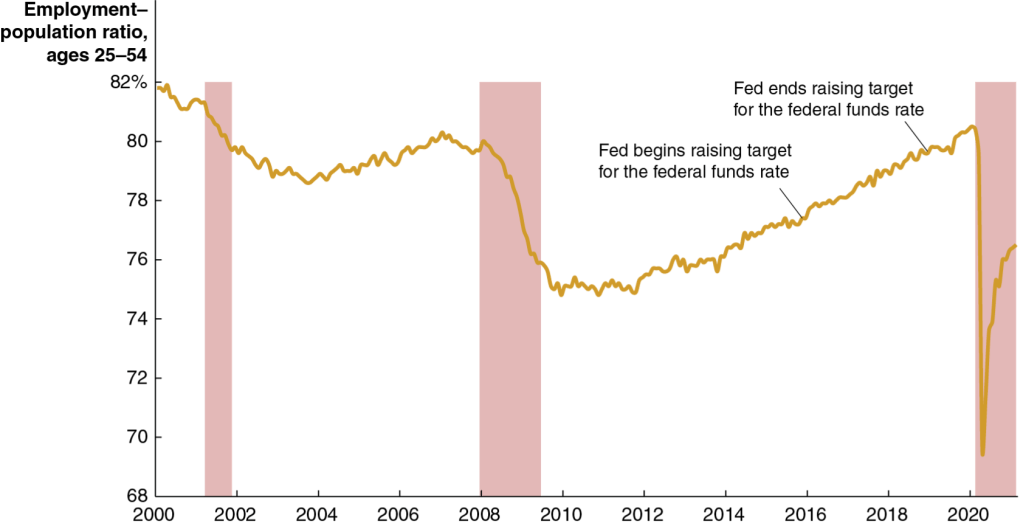
He used the following figure to illustrate his point.

Bostic interpreted the figure as follows:
“[The red areas in the figure are] periods of time when the actual unemployment rate fell below what the U.S. Congressional Budget Office now estimates as the so-called natural rate of unemployment. I refer to these episodes as “high-pressure” periods. Here is the punchline. Dating back to 1960, every high-pressure period ended in a recession. And all but one recession was preceded by a high-pressure period….
I think a risk management approach requires that we at least consider the possibility that unemployment rates that are lower than normal for an extended period are symptoms of an overheated economy. One potential consequence of overheating is that inflationary pressures inevitably build up, leading the central bank to take a much more “muscular” stance of policy at the end of these high-pressure periods to combat rising nominal pressures. Economic weakness follows [resulting typically, as indicated in the figure by the gray band, in a recession].”
By July 2019, a majority of the members of the FOMC, including Chair Powell, had come to believe that with no sign of inflation accelerating, they could safely cut the federal funds rate. But they had not yet explicitly abandoned the view that the FOMC should act to preempt increases in inflation. The formal change came in August 2020 when, as discussed earlier, the FOMC announced the new FAIT.
At the time the FOMC adopted its new monetary policy strategy, most members expected that any increase in inflation owing to problems caused by the Covid-19 pandemic—particularly the disruptions in supply chains—would be transitory. Because inflation has proven to be more persistent than Fed policymakers and many economists expected, two aspects of the FAIT approach to monetary policy have been widely discussed: First, the FOMC did not explicitly state by how much inflation can exceed the 2 percent target or for how long it needs to stay there before the Fed will react. The failure to elaborate on this aspect of the policy has made it more difficult for workers, firms, and investors to gauge the Fed’s likely reaction to the acceleration in inflation that began in the spring of 2021. Second, the FOMC’s decision to abandon the decades-long policy of preempting inflation may have made it more difficult to bring inflation down to the 2 percent target without causing a recession.
Federal Reserve Governor Lael Brainard recently remarked that “it is of paramount importance to get inflation down” and some Fed policymakers believe that the FOMC will have to begin increasing its target for the federal funds rate more aggressively. (The speech in which Governor Brainard discusses her current thinking on monetary policy can be found here.) For instance James Bullard, president of the Federal Reserve Bank of St. Louis, has argued in favor of raising the target to above 3 percent this year. With the Fed’s preferred measure of inflation running above 5 percent, it would take substantial increases int the target to achieve a positive real federal funds rate.
It is an open question whether Jerome Powell finds himself in a position similar to that of Paul Volcker in 1979: Rapid increases in interest rates may be necessary to keep inflation from accelerating, but doing so risks causing a recession. In a recent speech (found here), Powell pledged that: “We will take the necessary steps to ensure a return to price stability. In particular, if we conclude that it is appropriate to move more aggressively by raising the federal funds rate by more than 25 basis points at a meeting or meetings, we will do so.”
But Powell argued that the FOMC could achieve “a soft landing, with inflation coming down and unemployment holding steady” even if it is forced to rapidly increase its target for the federal funds rate:
“Some have argued that history stacks the odds against achieving a soft landing, and point to the 1994 episode as the only successful soft landing in the postwar period. I believe that the historical record provides some grounds for optimism: Soft, or at least softish, landings have been relatively common in U.S. monetary history. In three episodes—in 1965, 1984, and 1994—the Fed raised the federal funds rate significantly in response to perceived overheating without precipitating a recession.”
Some economists have been skeptical that a soft landing is likely. Harvard economist and former Treasury Secretary Lawrence Summers has been particularly critical of Fed policy, as in this Twitter thread. Summers concludes that: “I am apprehensive that we will be disappointed in the years ahead by unemployment levels, inflation levels, or both.” (Summers and Harvard economist Alex Domash provide an extended discussion in a National Bureau of Economic Research Working Paper found here.)
Clearly, we are in a period of great macroeconomic uncertainty.
Macro Solved Problems on Treasury Bonds and Defining Inflation

With the owners of the Major Labor Baseball teams and the Major League Players Association having finally settled on a new collective bargaining agreement, the baseball season will soon begin. Ernie Banks, the late Hall of Fame shortstop for the Chicago Cubs, was known for his upbeat personality. However bad the weather might be at Chicago’s Wrigley Field, Banks would run on the field and say, “What a great day for baseball! Let’s play two.”
In honor of Ernie Banks, today let’s do two Solved Problems in macro. They both involve errors that students in principles courses often make. So, in that sense they would also work as Don’t Let This Happen to You features.
Solved Problem 1.: Bond Yields and Bond Prices
An article in the Financial Times had the following headline: “U.S. Government Bond Prices Drop Ahead of Federal Reserve Meeting.” The first sentence of the article reads: “U.S. government bond yields rose to multiyear highs on Monday ahead of this week’s Federal Reserve meeting ….”
a. When a media article mentions “U.S. government bonds,” what type of bonds are they referring to?
b. Is there a contradiction between the headline and the first sentence of the article? Is the article telling us that U.S. government bonds went up or down? Briefly explain.
Solving the Problem
Step 1: Review the chapter material. This problem is about the inverse relationship between bond yields and bond prices, so you may want to review Macroeconomics, Chapter 6, Appendix, “Using Present Value” (Economics, Chapter 8, Appendix, “Using Present Value”). You may also want to review the discussion of U.S. Treasury bonds in Macroeconomics, Chapter 16, Section 16.6, “Deficits, Surpluses, and Federal Government Debt” (Economics, Chapter 26, Section 26.6, “Deficits, Surpluses, and Federal Government Debt”).
Step 2: Answer part a. by explaining what media articles are referring to when they use the phrase “U.S. government bonds.” As discussed in Chapter 16, Section 16.6, most of the bonds issued by the federal government of the United States are U.S. Treasury bonds. The Treasury sells these bonds to investors when the federal government doesn’t collect enough in tax revenues to pay for all of its spending. So, when the media refers to U.S. government bonds, without further explanation, the reference is always to U.S. Treasury bonds.
Step 3: Answer part b. by explaining that there is no contradiction between the headline and the first sentence of the article. An important fact about bond markets is that when the price of a bond falls, the yield—or interest rate—on the bond rises. The reverse is also true: When the price of a bond rises, the yield on the bond falls. The reason why this relationship holds is explained in the Appendix to Chapter 6: The price of a bond (or other financial asset) should be equal to the present value of the payments an investor receives from owning that asset. If you buy a U.S. Treasury bond, the price will equal the present value of the coupon payments the Treasury sends you during the life of the bond and the final payment to you by the Treasury of the principal, or face value of the bond. Remember that present value is the value in today’s dollars of funds to be received in the future. The higher the interest rate, the lower the present value of a payment to be received in the future. So a higher yield, or interest rate, on a bond results in a lower price of the bond because the higher yield reduces the present value of the payments to be received from the bond.
Therefore, whenever the yield on a bond rises, the price of the bond must fall (and whenever the yield on a bond falls, the price of the bond must rise. So, we can conclude that the headline of the Financial Times article and the first sentence of the article are consistent, not contradictory: Because the prices of Treasury bonds fell, the yields on the bonds must have risen.
Source: Nicholas Megaw, Naomi Rovnick, George Steer, and Hudson Lockett, “U.S. Government Bond Prices Drop Ahead of Federal Reserve Meeting,” ft.com, March 14, 2022.
Solved Problem 2: Being Careful about the Definition of Inflation
An article in the New York Times contrasted inflation during the 1970s with inflation today:
“Price increases had run high for more than a decade by the time Mr. Volcker became chair [of the Federal Reserve Board of Governors] in 1979 …. Shopper expected prices to go up, businesses knew that, and both acted accordingly. This time, inflation has been anemic for years (until recently), and most consumers and investors expect costs to return to lower levels before long, survey and market data show.”
a. What does the article mean by “inflation has been anemic for years”?
b. In the last sentence what “costs” is the article referring to?
c. Is the article correctly using the definition of inflation in the last sentence? Briefly explain.
Solving the Problem
Step 1: Review the chapter material. This problem is about the definition of inflation, so you may want to review Macroeconomics, Chapter 9, Section 9.4, “Measuring Inflation” (Economics, Chapter 20, Section 20.4, “Measuring Inflation”).
Step 2: Answer part a. by explaining what the phrase “inflation has been anemic for years” means. Anemia is a medical disorder that usually has the symptom of fatigue. So, the word “anemic” is often used to mean weak. The article is arguing that until recently, the inflation rate had been weak, or slow.
Step 3: Answer part b. by explaining what the article is referring to by “costs.” Economists typically use the word costs for the amount that firm pays to produce a good—labor costs, raw material costs, and so on. Here, though, the article is using “costs” to mean “prices.” Costs is often used this way in everyday conversation: “I didn’t buy a new car because they cost too much.” Or: “Has the cost of a movie ticket increased?”
Step 4: Answer part c. by explaining whether the article is correctly using the definition of inflation. In writing “consumers and investors expect costs to return to lower levels” the article is making a common mistake. The article seems to mean that consumers and investors expect that the rate of inflation will be lower in the future. But even if the rate of inflation declines from nearly 8 percent in early 2022 to, say, 3 percent in 2023, prices will still be increasing. So, prices (“costs” in the sentence) will still be higher next year even if the rate of inflation is lower. In other words, even if the rate of increase in prices—inflation—declines, the price level will still be higher.
It’s a common mistake to think that a decline in the inflation rate means that prices will be lower, when actually prices will still be increasing, just more slowly.
Source: Jeanna Smialek, “Powell Admires Volcker. He May Have to Act Like Him,” New York Times, March 14, 2022.
Inflation, Supply Chain Disruptions, and the Peculiar Process of Purchasing a Car

Inflation as measured by the percentage change in the consumer price index (CPI) from the same month in the previous year was 7.9 percent in February 2022, the highest rate since January 1982—near the end of the Great Inflation that began in the late 1960s. The following figure shows inflation in the new motor vehicle component of the CPI. The 12.4 percent increase in new car prices was the largest since April 1975.

The increase in new car prices was being driven partly by increases in aggregate demand resulting from the highly expansionary monetary and fiscal policies enacted in response to the economic disruptions caused by the Covid-19 pandemic, and partly from shortages of semiconductors and some other car components, which reduced the supply of new cars.
As the following figure shows, inflation in used car prices was even greater. With the exception of June and July of 2021, the 41.2 percent increase in used car prices in February 2022 was the largest since the Bureau of Labor Statistics began publishing these data in 1954.

Because used cars are a substitute of new cars, rising prices of new cars caused an increase in demand for used cars. In addition, the supply of used cars was reduced because car rental firms, such as Enterprise and Hertz, had purchased fewer new cars during the worst of the pandemic and so had fewer used cars to sell to used car dealers. Increased demand and reduced supply resulted in the sharp increase in the price of used cars.
Another factor increasing the prices consumers were paying for cars was a reduction in bargaining—or haggling—over car prices. Traditionally, most goods and services are sold at a fixed price. For example, some buying a refrigerator usually pays the posted price charged by Best Buy, Lowes, or another retailer. But houses and cars have been an exception, with buyers often negotiating prices that are lower than the seller was asking.
In the case of automobiles, by federal law, the price of a new car has to be posted on the car’s window. The posted price is called the Manufacturer’s Suggested Retail Price (MSRP), often referred to as the sticker price. Typically, the sticker price represents a ceiling on what a consumer is likely to pay, with many—but not all—buyers negotiating for a lower price. Some people dislike the idea of bargaining over the price of a car, particularly if they get drawn into long negotiations at a car dealership. These buyers are likely to pay the sticker price or something very close to it.
As a result, car dealers have an opportunity to practice price discrimination: They charge buyers whose demand for cars is more price elastic lower prices and buyers whose demand is less price elastic higher prices. The car dealers are able to separate the two groups on the basis of the buyers willingness to haggle over the price of a car. (We discuss price discrimination in Microeconomics and Economics, Chapter 15, Section 15.5.) Prior to the Covid-19 pandemic, the ability of car dealers to practice this form of price discrimination had been eroded by the availability of online car buying services, such as Consumer Reports’ “Build & Buy Service,” which allow buyers to compare competing price offers from local car dealers. There aren’t sufficient data to determine whether using an online buying service results in prices as low as those obtained by buyers willing to haggle over price face-to-face with salespeople in dealerships.
In any event, in 2022 most car buyers were faced with a different situation: Rather than serving as a ceiling on the price, the MSRP, had become a floor. That is, many buyers found that given the reduced supply of new cars, they had to pay more than the MSRP. As one buyer quoted in a Wall Street Journal article put it: “The rules have changed so dramatically…. [T]he dealer’s position is ‘This is kind of a take-it-or-leave-it proposition.’” According to the website Edmunds.com, in January 2021, only about 3 percent of cars were sold in the United States for prices above MSRP, but in January 2022, 82 percent were.
Car manufacturers are opposed to dealers charging prices higher than the MSRP, fearing that doing so will damage the car’s brand. But car manufacturers don’t own the dealerships that sell their cars. The dealerships are independently owned businesses, a situation that dates back to the beginning of the car industry in the early 1900s. Early automobile manufacturers, such as Henry Ford, couldn’t raise sufficient funds to buy and operate a nationwide network of car dealerships. The manufacturers often even had trouble financing the working capital—or the funds used to finance the daily operations of the firm—to buy components from suppliers, pay workers, and cover the other costs of manufacturing automobiles.
The manufacturers solved both problems by relying on a network of independent dealerships that would be given franchises to be the exclusive sellers of a manufacturer’s brand of cars in a given area. The local businesspeople who owned the dealerships raised funds locally, often from commercial banks. Manufacturers generally paid their suppliers 30 to 90 days after receiving shipments of components, while requiring their dealers to pay a deposit on the cars they ordered and to pay the balance due at the time the cars were delivered to the dealers. One historian of the automobile industry described the process:
The great demand for automobiles and the large profits available for [dealers], in the early days of the industry … enabled the producers to exact substantial advance deposits of cash for all orders and to require cash payment upon delivery of the vehicles …. The suppliers of parts and materials, on the other hand, extended book-account credit of thirty to ninety days. Thus the automobile producer had a month or more in which to assemble and sell his vehicles before the bills from suppliers became due; and much of his labor costs could be paid from dealers’ deposits.
The franchise system had some drawbacks for car manufacturers, however. A car dealership benefits from the reputation of the manufacturer whose cars it sells, but it has an incentive to free ride on that reputation. That is, if a local dealer can take an action—such as selling cars above the MSRP—that raises its profit, it has an incentive to do so even if the action damages the reputation of Ford, General Motors, or whichever firm’s cars the dealer is selling. Car manufacturers have long been aware of the problem of car dealers free riding on the manufacturer’s reputation. For instance, in the 1920s, Ford sent so-called road men to inspect Ford dealers to check that they had clean, well-lighted showrooms and competent repair shops in order to make sure the dealerships weren’t damaging Ford’s brand.
As we discuss in Microeconomics and Economics, Chapter 10, Section 10.3, consumers often believe it’s unfair of a firm to raise prices—such as a hardware store raising the prices of shovels after a snowstorm—when the increases aren’t the result of increases in the firm’s costs. Knowing that many consumers have this view, car manufacturers in 2022 wanted their dealers not to sell cars for prices above the MSRP. As an article in the Wall Street Journal put it: “Historically, car companies have said they disapprove of their dealers charging above MSRP, saying it can reflect poorly on the brand and alienate customers.”
But the car manufacturers ran into another consequence of the franchise system. Using a franchise system rather than selling cars through manufacturer owned dealerships means that there are thousands of independent car dealers in the United States. The number of dealers makes them an effective lobbying force with state governments. As a result, most states have passed state franchise laws that limit the ability of car manufacturers to control the actions of their dealers and sometimes prohibit car manufacturers from selling cars directly to consumers. Although Tesla has attained the right in some states to sell directly to consumers without using franchised dealers, Ford, General Motors, and other manufacturers still rely exclusively on dealers. The result is that car manufacturers can’t legally set the prices that their dealerships charge.
Will the situation of most people paying the sticker price—or more—for cars persist after the current supply chain problems are resolved? AutoNation is the largest chain of car dealerships in the United States. Recently, Mike Manley, the firm’s CEO, argued that the substantial discounts from the sticker price that were common before the pandemic are a thing of the past. He argued that car manufacturers were likely to keep production of new cars more closely in balance with consumer demand, reducing the number of cars dealers keep in inventory on their lots: “We will not return to excessively high inventory levels that depress new-vehicle margins.”
Only time will tell whether the situation facing car buyers in 2022 of having to pay prices above the MSRP will persist.
Sources: Mike Colias and Nora Eckert, “A New Brand of Sticker Shock Hits the Car Market,” Wall Street Journal, February 26, 2022; Nora Eckert and Mike Colias, “Ford and GM Warn Dealers to Stop Charging So Much for New Cars,” Wall Street Journal, February 9, 2022; Gabrielle Coppola, “Car Discounts Aren’t Coming Back After Pandemic, AutoNation Says,” bloomberg.com, February 9, 2022; cr.org/buildandbuy; Lawrence H. Seltzer, A Financial History of the American Automobile Industry, Boston: Houghton-Mifflin, 1928; and Federal Reserve Bank of St. Louis.
Would Cutting the Federal Excise Tax on Gasoline Lower the Price that Consumers Pay?

The federal government levies an excise tax of 18.4 cents per gallon of gasoline. (An excise tax is a tax that a government imposes on a particular product. In addition to the tax on gasoline, the federal government imposes excise taxes on tobacco, alcohol, airline tickets, and a few other products.) In February 2022, inflation was running at the highest level in several decades. The average retail price of gasoline across the country had risen to $3.50 per gallon from $2.60 per gallon a year earlier. The following figure shows fluctuations in the retail price of gasoline since January 2000.

Policymakers were looking for ways to lessen the effects of inflation on consumers. An article in the Wall Street Journalreported that several Democratic members of the U.S. Senate, including Mark Kelly of Arizona, Maggie Hassan of New Hampshire, and Raphael Warnock of Georgia proposed that the federal excise tax on gasoline be suspended for the remainder of 2022. The sponsors of the proposal believed that cutting the tax would reduce the price of gasoline that consumers pay at the pump. Other members of the Senate weren’t so sure, with one quoted as saying that cutting the tax was “not going to change anything” and another arguing that oil companies would receive most of the benefit of the tax cut.
Some members of Congress were opposed to suspending the gasoline tax because the revenue raised from the tax is placed in the highway trust fund, which helps to pay for federal contributions to highway building and repair and for mass transit. In that sense, the gasoline tax follows the benefits-received principle, under which people who receive benefits from a government program—in this case, highway maintenance—should help pay for the program. (We discuss the principles for evaluating taxes in Microeconomics, Chapter 17, Section 17.2 and in Economics, Chapter 17, Section 17.2) Other members of Congress were opposed to suspending the tax because they believe that the tax helps to reduce the quantity of gasoline consumed, thereby helping to slow climate change.
Focusing just on the question of the effect of suspending the tax on the retail price of gasoline, what can we conclude? The question is one of tax incidence, which looks at the actual division of the burden of a tax between buyers and sellers in a market. In other words, tax incidence looks beyond the fact that gasoline stations collect the tax and send the revenue to federal government to the issue of who actually pays the tax. As we note in Chapter 17, Section 17.3:
When the demand for a product is less elastic than supply, consumers pay the majority of the tax on the product. When the demand for a product is more elastic than supply, firms pay the majority of the tax on the product.
Consumers would receive all of the tax cut—that is, the retail price of gasoline would fall by 18.4 cents—only in the polar case where the demand for gasoline were perfectly price inelastic. Similarly, consumers would receive none of the tax cut and the price of gasoline would remain unchanged—so oil companies would receive all of the tax cut—only in the polar case where the demand for gasoline is perfectly price inelastic. (It’s a worthwhile exercise to show these two cases using demand and supply graphs.)
In the real world, we would expect to be somewhere in between these two cases, with consumers receiving some of the benefit of suspending the tax and producers receiving the remainder of the benefit. The short-run price elasticity of demand for gasoline is quite small; according to one estimate it is only −.06. The short-run price elasticity of supply of gasoline is likely to be somewhat larger than that in absolute value, which means that we would expect that consumers would receive the majority of the tax cut. (Note that we would expect the long-run price elasticities of demand and supply to both be larger for reasons we discuss in Chapter 6, Section 6.2 and 6.6.) In other words, the retail price of gasoline would fall, holding all other factors constant, but not by the full tax cut of 18.4 cents.
Joseph Doyle of MIT and Krislert Samphantharak of the University of California, San Diego studied the effect of suspension in the state excise tax on gasoline in Indiana and Illinois in 2000. In that year, Indiana suspended collecting its gasoline excise tax for 120 days and Illinois suspended its tax for 184 days. The authors estimate that consumers received about 70 percent of the tax cut in the form of lower gasoline prices. If we apply that estimate to the federal gasoline tax, then suspending the tax would lower the price of gasoline by about 12.9 cents per gallon, holding all other factors that affect the price of gasoline constant. As the above figure shows, the retail price of gasoline frequently fluctuates up and down by more than 12.9 cents, even over fairly brief periods of time. In that sense, the effect on the gasoline market of suspending the federal excise tax on gasoline would be relatively small.
Sources: Andrew Duehren and Richard Rubin, “Some Lawmakers Want to Halt Gas Tax Amid High Inflation. Others See a Gimmick,” Wall Street Journal, February 16, 2022; Tony Romm and Jeff Stein, “White House, Congressional Democrats Eye Pause of Federal Gas Tax as Prices Remain High, Election Looms,” Washington Post, February 15, 2022; Joseph J. Doyle, Jr., Krislert Samphantharak, “$2.00 Gas! Studying the Effects of a Gas Tax Moratorium,” Journal of Public Economics, Vol. 92, No.s 3-4, April 2008, pp. 869-884; and Federal Reserve Bank of St. Louis.
Are Economic Profits a Sign of Market Power?

An article in the Washington Post discussed a debate among President Biden’s economic advisers. The debate was over “over whether the White House should blame corporate consolidation and monopoly power for price hikes.” Some members of the National Economic Council supported the view that the increase in inflation that began in the spring of 2021 was the result of a decline in competition in the U.S. economy.
Some Democratic members of Congress have also supported this view. For instance, Massachusetts Senator Elizabeth Warren argued on Twitter that: “One clear explanation for higher inflation? Giant corporations are exploiting their market power to further raise prices. And corporate executives are bragging about their higher profits.” Or, as Vermont Senator Bernie Sanders put it: “The problem is not inflation. The problem is corporate greed, collusion & profiteering.”
But according to the article, Cecilia Rouse, chair of the President’s Council of Economic Advisers (CEA), and other members of the CEA are skeptical that a lack of competition are the main reason for the increase in inflation, arguing that very expansionary monetary and fiscal policies, along with disruptions to supply chains, have been more important.
In an earlier blog post (found here), we noted that a large majority of more than 40 well-known academic economists surveyed by the Booth School of Business at the University of Chicago disagreed with the statement: “A significant factor behind today’s higher US inflation is dominant corporations in uncompetitive markets taking advantage of their market power to raise prices in order to increase their profit margins.”
One difficulty with the argument that the sharp increase in inflation since mid-2021 was due to corporate greed is that there is no particular reason to believe that corporations suddenly became more greedy than they had been when inflation was much lower. If inflation were mainly due to corporate greed, then greed must fluctuate over time, just as inflation does. Economic writer and blogger Noah Smith poked fun at this idea in the following graph.

It’s worth noting that “greed” is one way of characterizing the self-interested behavior that underlies the assumption that firms maximize profits and individual maximize utility. (We discuss profit maximization in Microeconomics, Chapter 12, Section 12.2, and utility maximization in Chapter 10, Section 10.1.) When economists discuss self-interested behavior, they are not making a normative statement that it’s good for people to be self-interested. Instead, they are making a positive statement that economic models that assume that businesses maximize profit and consumers maximize utility have been successful in analyzing and predicting the behavior of businesses and households.
Corporate profits increased from $1.95 trillion in the first quarter of 2021 to $2.40 trillion in third quarter of 2021 (the most recent quarter for which data are available). Using another measure of profit, during the same period, corporate profits increased from about 16 percent of value added by nonfinancial corporate businesses to about 18 percent. (Value added measures the market value a firm adds to a product. We discuss calculating value added in Macroeconomics, Chapter 8, Section 8.1.)
There have been mergers in some industries that may have contributed to an increase in profits—the Biden Administration has singled out mergers in the meatpacking industry as having led to higher beef and chicken prices. At this point, though, it’s not possible to gauge the extent to which mergers have been responsible for higher prices, even in the meatpacking industry.
An increase in profit is not by itself an indication that firms have increased their market power. We would expect that even in a perfectly competitive industry, an increase in demand will lead in the short run to an increase in the economic profit earned by firms in the industry. But in the long run we expect economic profit to be competed away either by existing firms expanding their production or by new firms entering the industry.
In Chapter 12, we use Figure 12.8 to illustrate the effects of entry in the market for cage-free eggs. Panel (a) shows the market for cage-free eggs, made up of all the egg sellers and egg buyers. Panel (b) shows the situation facing one farmer producing cage-free eggs. (Note the very different scales of the horizontal axes in the two panels.) At $3 per dozen eggs, the typical egg farmer is earning an economic profit, shown by the green rectangle in panel (b). That economic profit attracts new entrants to the market—perhaps, in this case, egg farmers who convert to using cage-free methods. The result of entry is a movement down the demand curve to a new equilibrium price of $2 per dozen. At that price, the typical egg farmer is no longer earning an economic profit.

A few last observations:
- The recent increase in profits may also be short-lived if it reflects a temporary increase in demand for some durable goods, such as furniture and appliances, raising their prices and increasing the profits of firms that produce them. The increase in spending on goods, and reduced spending on services, appears to have resulted from: (1) Households having additional funds to spend as a result of the payments they received from fiscal policy actions in 2020 and early 2021, and (2) a reluctance of households to spend on some services, such as restaurant meals and movie theater tickets, due to the effects of the Covid-19 pandemic.
- The increase in profits in some industries may also be due to a reduction in supply in those industries having forced up prices. For instance, a shortage of semiconductors has reduced the supply of automobiles, raising car prices and the profits of automobile manufacturers. Over time, supply in these industries should increase, bringing down both prices and profits.
- If some changes in consumer demand persist over time, we would expect that the economic profits firms are earning in the affected industries will attract the entry of new firms—a process we illustrated above. In early 2022, this process is far from complete because it takes time for new firms to enter an industry.
Source: Jeff Stein, “White House economists push back against pressure to blame corporations for inflation,” Washington Post, February 17, 2022; Mike Dorning, “Biden Launches Plan to Fight Meatpacker Giants on Inflation,” bloomberg.com, January 3, 2022; and U.S. Bureau of Economic Analysis.ec
Does Inflation Affect Lower-Income People More than Higher-Income People?
There’s a consensus among economists that increases in unemployment during a recession typically are larger for lower-income people than for higher-income people. Lower-income people are more likely to hold jobs requiring fewer skills and firms typically expect that when they lay off less-skilled workers during a recession they will be able to higher them—or other workers with similar skills—back after the recession ends. Because higher income have skills that may be difficult to replace, firms are more reluctant to lay them off.
For instance, in an earlier blog post (found here) we noted that during the period in 2020 when many restaurants were closed, the Cheesecake Factory continued to pay its 3,000 managers while it laid off most of its servers. That strategy made it easier for the restaurant chain to more easily expand its operations when the worst of government-ordered closures were over. More generally, Serdar Birinci and YiLi Chien of the Federal Reserve Bank of St. Louis found that workers in the lowest 20 percent (or quintile) of earnings experienced an increased unemployment rate from 4.4 percent in January 2020 to 23.4 percent in April 2020, whereas workers in the highest quintile of earnings experienced an increase only from 1.1 percent in January to 4.8 percent in April.
If lower-income people are hit harder by unemployment, are they also hit harder by inflation? Answering that question is difficult because the U.S. Bureau of Labor Statistics (BLS) doesn’t routinely release data on inflation in the prices of goods and services purchased by households at different income levels. The main measure of consumer price inflation compiled by the BLS represents changes in the consumer price index (CPI). The CPI is an index of the prices in a market basket of goods and services purchased by households living in urban areas. The information on consumer purchases comes from interviews the BLS conducts every three months with a sample of consumers and from weekly diaries in which a sample of consumers report their purchases. (We discuss the CPI in Macroeconomics, Chapter 9, Section 9.4 and in Economics, Chapter 19, Section 19.4.)
The BLS releases three measures of the CPI, the two most widely used of which are the CPI-U for all urban consumers and CPI-W for urban wage earners. CPI-W covers the subset of households that receive at least half their household income from clerical or wage occupations and who have at least one wage earner who worked for 37 weeks or more during the previous year. CPI-U represents about 93 percent of the U.S. population and CPI-W represents about 29 percent of the U.S. population. Finally, in 1988 Congress instructed the BLS to compile a consumer price index reflecting the purchases of people aged 62 and older. This version of the CPI is labeled R-CPI-E; the R indicates that it is a research series and the E indicates that it is intended to measure the prices of goods and services purchased by elderly people. Because the sample used to calculate the R-CPI-E is relatively small and because of some other difficulties that may reduce the accuracy of the index, the BLS considers it a series best suited for research and does not include the data in its monthly “Consumer Price Index” publication. In any event, as the following figure shows, inflation, measured as the percentage change in the CPI from the same month in the previous year, has been very similar for all three measures of the CPI.

Because the market baskets of goods and services consumed by a mix of high and low-income households is included in all three versions of the CPI, none of the versions provides a way to measure the possibly different effects of inflation on low-income and on high-income households. A study by Josh Klick and Anya Stockburger of the BLS attempts to fill this gap by constructing measures of the CPI for low-income and for high-income households. They define low-income households as those in the bottom 25 percent (quartile) of the income distribution and high-income households as those in the top quartile of the income distribution. During the time period of their analysis—December 2003 to December 2018—the bottom quartile had average annual incomes of $12,705 and the top quartile had average annual incomes of $155,045.
The BLS researchers constructed market baskets for the two groups. The expenditure weights—representing the mix of products purchased—don’t differ too strikingly between lower-income and higher-income households, as the figure below shows. The largest differences are housing, with low-income households having a market basket weight of 45.2 percent and high-income households having a market basket weight of 39.5 percent, and transportation, with low-income households having a market basket weight of 13.0 percent and high-income households having a market basket weight of 17.2 percent.

The following table shows the inflation rate as measured by changes in different versions of the CPI over the period from December 2003 to December 2018. During this period, the CPI-U (the version of the CPI that is most frequently quoted in news stories) increased at an annual rate of 2.1 percent, which was the same rate as the CPI-W. The R-CPI-E increased at a slightly faster rate of 2.2 percent. Lower-income households experienced the highest inflation rate at 2.3 percent and higher-income households experienced the lowest inflation rate of 2.0 percent.
| CPI-U | CPI-W | R-CPI-E | CPI for lowest income quartile | CPI for highest income quartile |
| 2.1% | 2.2% | 2.1% | 2.3% | 2.0% |
The differences in inflation rates across groups were fairly small. Can we conclude that the same was true during the recent period of much higher inflation rates? We won’t know with certainty until the BLS extends its analysis to cover at least the years 2021 and 2022. But we can make a couple of relevant observations. First, for many people the most important aspect of inflation is whether prices are increasing faster of slower than their wages. In other words, people are interested in what is happening to their real wage. (We discuss calculating real wage rates in Macroeconomics, Chapter 9, Section 9.5 and in Economics, Chapter 19, Section 19.5.)
The Federal Reserve Bank of Atlanta compiles data on wage growth, including wage growth by workers in different income quartiles. The following figure shows that workers in the top quartile have experienced more rapid wage growth in the months since the beginning of the Covid-19 pandemic than have workers in the other quartiles. This gap continues a trend that began in 2015. The bottom quartile has experienced the slowest rate of income growth. (Note that the researchers at the Atlanta Fed compute wage growth as a 12-month moving average rather than as the percentage from the same month in the previous year, as we have been doing when calculating inflation using the CPI.) For example, in January 2022, calculated this way, average wage growth in the top quartile was 5.8 percent as opposed to 2.9 percent in the bottom quartile.

As with any average, there is some variation in the experiences of different individuals. Although, as a group, lower-income workers have seen wage growth that lags behind other workers, in some industries that employ many lower-income people, wage growth has been strong. For instance, as measured by average hourly earnings, wages for all workers in the private sector increased by 5.7 percent between January 2021 and 2022. But average hourly earnings in the leisure and hospitality industry—which employs many lower-income workers—increased by 13.0 percent.
Overall, it seems likely that the real wages of higher-income workers have been increasing while the real wages of lower-income workers have been decreasing, although the experience of individual workers in both groups may be very different than the average experience.
Sources: Josh Klick and Anya Stockburger, “Experimental CPI for Lower and Higher Income Households Serdar,” U.S. Bureau of Labor Statistics, Working Paper 537, March 8, 2021; Birinci and YiLi Chien, “An Uneven Crisis for Lower-Income Households,” Federal Reserve Bank of St. Louis, Annual Report 2020, April 7, 2021; and Federal Reserve Bank of Atlanta, “Wage Growth Tracker,” https://www.atlantafed.org/chcs/wage-growth-tracker.
Inflation, Interest Rates, and Stock Prices
Caution: Long post!
An article in the Wall Street Journal quoted an economist at a financial services firm as noting that strong growth in wages could lead to sustained inflation. The article stated that as a result “the yield on the 10-year U.S. Treasury note [rose to] within reach of 2%” and that: “Rising [bond] yields this year have rattled markets and hurt tech stocks in particular ….”
What are the links between wage inflation and price inflation, inflation and bond yields, and bond yields and stock prices—particularly the prices of tech stocks?
The link between wage inflation and price inflation. The monthly “Employment Situation” reports from the Bureau of Labor Statistics (BLS), in addition to providing data on payroll employment and the unemployment rate, also provide data on average hourly earnings (AHE). AHE are the wages and salaries per hour worked that private, nonfarm business pay workers. AHE don’t include the value of benefits that firms provide workers, such as contributions to 401(k) retirement accounts or health insurance. The following figure shows changes in AHE from the same month in the previous year. The figure shows that since the Covid-19 pandemic first began to affect the U.S. economy in March 2020, AHE have moved erratically. But since the fall of 2021, growth in AHE has been consistently above the 2 percent to 4 percent range that prevailed in the years after the end of the Great Recession of 2007–2009.

Employee compensation is the largest cost for most firms. For the economy as whole, employee compensation is about 80 percent of total costs. When firms pay higher wages per hour, their costs per unit of output don’t rise unless the wage increases are greater than the rate of growth of labor productivity, or output per hour worked. Increases in wages in the range of 5 percent to 6 percent are well above the rate of growth of labor productivity and, so, firms are likely to pass through the wage increases by raising prices. Note that the higher prices may prompt workers to push for higher wage increases to offset the decline in the real purchasing power of their wages, potentially setting off a wage-price spiral. (We discussed the possibility of a wage-price spiral in a recent post here.)
The link between inflation and bond yields. When investors lend money by, for instance, buying a bond, they are concerned with the interest rate they will receive after correcting for the effects of inflation. In other words, they focus on the real interest rate, which is equal to the nominal interest rate, or the stated interest rate on the loan or bond, minus the expected inflation rate:
Real interest rate = Nominal interest rate – Expected inflation rate.
We can rewrite this relationship as:
Nominal interest rate = Real interest rate + Expected inflation rate.
The second equation indicates that if investors expect the inflation rate to increase, then, unless the real interest rate changes, the nominal interest rate will increase. The Fisher effect is the idea associated with Yale economist Irving Fisher that the nominal interest rate rises or falls by the same number of percentage points as the expected inflation rate. So, for instance, if investors expect that the inflation rate will increase from 3 percent to 5 percent, then the nominal interest rate will also increase by two percentage points.
Because of real-world frictions, such as the broker fees that investors pay when buying and selling bonds and the taxes investors pay when they sell a bond that has increased in price, the Fisher effect doesn’t hold exactly. Still, most economists agree that an increase in the expected inflation rate will cause an increase in nominal interest rates. The following figure shows movements in the interest rate on 10-year Treasury notes (blue line) and in inflation (red line). Note that, roughly speaking, the interest rate on the 10-year Treasury note is higher when inflation is higher and lower when inflation is lower. (We discuss real and nominal interest rates in Macroeconomics, Chapter 9, Section 9.6 and in Economics, Chapter 19, Section 19.6. We discuss the Fisher effect in Money, Banking, and the Financial System, Chapter 4, Section 4.3.)

The link between bond yields and stock prices. As wage inflation leads to price inflation and price inflation leads to higher interest rates on bonds—particularly U.S. Treasury bonds—why might stock prices be affected? First, investors consider U.S. Treasury bonds to be default risk free, which means that investors are certain that the Treasury will make the interest and principal payments on the bonds. Stock investments are much riskier because they depend on the future profits of the firms issuing the stocks and those profits may fluctuate in ways that are difficult for investors to anticipate. So as interest rates on Treasury bonds increase, some investors will decide to sell stocks and buy bonds, which will cause a decline in stock prices.
Second, most people value funds they will receive now or soon more highly than funds they will receive in the more distant future. For instance, if someone offered to pay you $1,000 today or $1,000 one year from now, you will prefer to receive the money today. In other words, the present value, or value today, of a payment you won’t receive until the future is worth less than the face value of the payment. For instance, the present value of $1,000 you won’t receive for a year is worth less than $1,000 in present value. The higher the interest rate is, the lower the present value of payments, such as dividends, that you will receive in the future.
Economists believe that price of a financial investment, like a bond or a stock, is equal to the present value of the payments you will receive from owning the asset. If you own a bond, you will receive interest payments and payment of the bond’s principal when the bond matures. If you own a stock, you will receive dividends, which are the payments that firms make to shareholders from the firms’ profits. Therefore stock prices should reflect the present value of the dividends that investors expect to receive from owning the stock. (We discuss present value and the relationship between interest rates and stock and bond prices in Macroeconomics, Chapter 6, Appendix, in Economics, Chapter 8, Appendix, and, more completely, in Money, Banking, and the Financial System, Chapter 3, Section 3.2 and Chapter 6, Section 6.2.)
The Wall Street Journal article we quoted above notes that the rising interest rate on the 10-year Treasury note was causing price declines in tech stocks in particular. The explanation is that tech firms often go through an initial period in which they may make very low profits or even suffer losses. Investors may still be willing to buy stock in tech firms because they expect the firms eventually to increase their profits and the dividends they pay. But because those profits will be earned in the future—often after a period of losses that may stretch for years—the present value of the profits and, therefore, the price of the stock depends more on the interest rate than would be true of a firm making breakfast cereal or frozen pizza that will be steadily earning profits through the years. Therefore, we would expect, as the article indicates, that the prices of tech firms are more likely to decline—or to decline more—when interest rates rise than is true of other firms.
The following figure shows the interest rate on the 10-year Treasury note (blue line with scale given on the left) and the values of the Nasdaq composite stock index (red line with the value for January 1, 2010 set equal to 100 and the scale given on the right). The Nasdaq includes the stocks of more tech firms than is true of the other widely followed stock market indexes—the S&P 500 and the Dow Jones Industrial Average. The figure shows that the declining interest rate on 10-year Treasury notes that began in late 2018 and continued through mid-2020 coincided with increases in the prices of the stocks in the Nasdaq index—apart from the spring of 2020 during the beginning of the Covid-19 pandemic. The most recent period shows that increases in the interest rate on the 10-year Treasury note have corresponded with a decline in the Nasdaq, as noted in the article.

Source: Sam Goldfarb, “Elevated Bond Yields Approach Key Milestone,” Wall Street Journal, February 7, 2022; U.S. Bureau of Economic Analysis, “Prices, Costs, and Profit per Unit of Real Gross Value Added of Nonfinancial Domestic Corporate Business,” January 27, 2022; and Federal Reserve Bank of St. Louis.
The Surprisingly Strong Employment Report for January 2022

The Bureau of Labor Statistics’ monthly report on the “Employment Situation” is generally considered the best source of information on the current state of the labor market. As we discuss in Macroeconomics, Chapter 9, Section 9.1 (and in Economics, Chapter 19, Section 19.1), economists, policymakers, and investors generally focus more on the establishment survey data on total payroll employment than on the household survey data on the unemployment rate. The initial data on employment from the establishment survey are subject to substantial revisions over time (we discuss this point further below). But the establishment survey has the advantage of being determined by data taken from actual payrolls rather than by unverified answers to survey questions, as is the case with the household survey data.
The establishment survey data for January 2022 (released on February 4, 2022) showed a surprisingly large increase in employment of 467,000. The consensus forecast had been for a significantly smaller increase of 150,000, with many economists expecting that the data would show a decrease in employment. The establishment survey is collected for pay periods that include the 12th of the month. In January 2022, in many places in the United States that pay period coincided with the height of the wave of infections from the Omicron variant of Covid-19. And, in fact, according to the household survey, the number of people out of work because of illness was 3.6 million in January—the most during the Covid-19 pandemic. So it seemed likely that payroll employment would have declined in January. But despite the difficulties caused by the pandemic, payroll employment increased substantially, likely reflecting firms’ continuing high demand for workers—a demand reflected in the very high level of job openings.
The employment report includes the BLS’s annual data revisions, which are based on a comprehensive payroll count for a particular month in the previous year—in this case, March 2021. The revisions also incorporate changes to the BLS’s seasonal adjustment factors. Each month, the BLS adjusts the raw payroll employment data to reflect seasonal fluctuations such as occur during and after the end-of-year holiday period. For instance, the change from December 2020 to January 2021 in the raw employment data was −2,824,000, whereas the adjusted change was 467,000 (as noted earlier). Obviously this difference is very large and is attributable to the BLS’s seasonal adjustments removing the employment surge in December attributable to seasonal hiring by retail stores, delivery firms, and other businesses strongly affected by the holidays.
The changes to the seasonal adjustment factors made the revisions to the 2021 payroll employment numbers unusually large. For instance, the BLS initially reported that employment increased from June 2021 to July 2021 by 1,091,000, whereas the revision reduced the increase to 689,000. Table A below is reproduced from the BLS report; the figure below the table shows the changes in employment from the previous month as originally published and as revised in the January report. Overall, the BLS revisions now show that employment increased by 217,000 more from 2020 to 2021 than initially estimated. The BLS expressed the opinion that: “Going forward, the updated models should produce more reliable estimates of seasonal movements. [Because there are now] more monthly observations related to the historically large job losses and gains seen in the pandemic-driven recession and recovery, the models can better distinguish normal seasonal movements from underlying trends.”


Source: The BLS “Employment Situation” report can be found here.
1/25/22 Podcast – Authors Glenn Hubbard & Tony O’Brien discuss inflation, inflation, inflation.
Authors Glenn Hubbard and Tony O’Brien as they talk about the leading economic issue of early 2022 – inflation! They discuss the resurgence of inflation to levels not seen in 40 years due to a combination of miscalculations in monetary and fiscal policy. The role of Quantitative Easing (QE) – and its future – is discussed in depth. Listen today to gain insights into the economic landscape.