A unicorn is a startup, or newly formed firm, that has yet to begin selling stock publicly and has a value of $1 billion or more. (We discuss the difference between private firms and public firms in Economics and Microeconomics, Chapter 8, chapter opener and Section 8.2, and in Macroeconomics, Chapter 6, chapter opener and Section 6.2.) Usually, when we think of unicorns, we think of tech firms. That assumption is largely borne out by the following list of the 10 highest-valued U.S.-based startups, as compiled by cbinsights.com.
Firm
Value
SpaceX
$100.3 B
Stripe
$95 B
Epic Games
$42 B
Instacart
$39 B
Databricks
$38 B
Fanatics
$27 B
Chime
$25 B
Miro
$17.5 B
Ripple
$15 B
Plaid
$13.4 B
Nine of the ten firms are technology firms, with six being financial technology—fintech—firms. (We discuss fintech firms in the Apply the Concept, “Help for Young Borrowers: Fintech or Ceilings on Interest Rates,” which appears in Macroeconomics, Chapter 14, Section 14.3, and Economics, Chapter 24, Section 24.3.) The one non-tech firm on the list is Fanatics, whose main products are sports merchandise and sports trading cards. Because a unicorn doesn’t issue publicly traded stock, the firm’s valuation is determined by how much an investor pays for a percentage of the firm. In Fanatics’s case, the valuation was based on a $1.5 billion investment in the firm made in early March 2022 by a group of investors, including Fidelity, the large mutual find firm; Blackrock, the largest hedge fund in the world; and Michael Dell, the founder of the computer company.
These investors were expecting that Fanatics would earn an economic profit. But, as we discuss in Chapter 14, Section 14.1 and Chapter 15, Section 15.2, a firm will find its economic profit competed away unless other firms that might compete against it face barriers to entry. Although Fanatics CEO Michael Rubin has plans for the firm to expand into other areas, including sports betting, the firm’s core businesses of sports merchandise and trading cards would appear to have low barriers to entry. There are already many firms selling sportswear and there are many firms selling trading cards. The investment required to establish another firm to sell those products is low. So, we would expect competition in the sports merchandise and trading card markets to eliminate economic profit.
The key to Fanatics success is that it is selling differentiated products in those markets. Its differentiation is based on a key resource that competitors lack access to: The right to produce sportswear with the emblems of professional sports teams and the right to produce trading cards that show images of professional athletes. Fanatics has contracts with the National Football League (NFL), Major League Baseball (MLB), the National Hockey League (NHL), the National Basketball Association (NBA), and Major League Soccer (MLS)—the five most important professional sports leagues in North America—to produce jerseys, caps, and other sportswear that uses the copyrighted brands of the leagues’ teams. (In some cases, as with the NBA, Fanatics shares the right with another firm.)
Similarly, Fanatics has the exclusive right to produce trading cards bearing the images of NFL, NBA, and MLB players. In January 2022, Fanatics bought Topps, the firm that for decades had held the right to produce MLB trading cards.
Fanatics has paid high prices to these sports leagues and their players to gain the rights to sell branded merchandise and cards. Some business analysts questioned whether Fanatics will be able to sell the merchandise and cards for prices high enough to earn an economic profit on its investments. Fanatics CEO Rubin is counting on an increase in the popularity of trading cards and the increased interest in sports caused by more states legalizing sports gambling.
That Fanatics has found a place on the list of the most valuable startups that is otherwise dominated by tech firms indicates that many investors agree with Rubin’s business strategy.
Sources: “The Complete List of Unicorn Companies,” cbinsights.com; Miriam Gottfried and Andrew Beaton, “Fanatics Raises $1.5 Billion at $27 Billion Valuation,” Wall Street Journal, March 2, 2022; Tom Baysinger, “Fanatics Scores $27 Billion Valuation,” axios.com March 2, 2022; Lauren Hirsch, “Fanatics Is Buying Mitchell & Ness, a Fellow Sports Merchandiser,” New York Times, February 18, 2022; and Kendall Baker, “Fanatics Bets Big on Trading Card Boom,” axios.com, January 5, 2022.
Supports: Macroeconomics, Chapter 10, Section 10.5, Economics Chapter 20, Section 20.5, and Essentials of Economics, Chapter 14, Section 14.2.
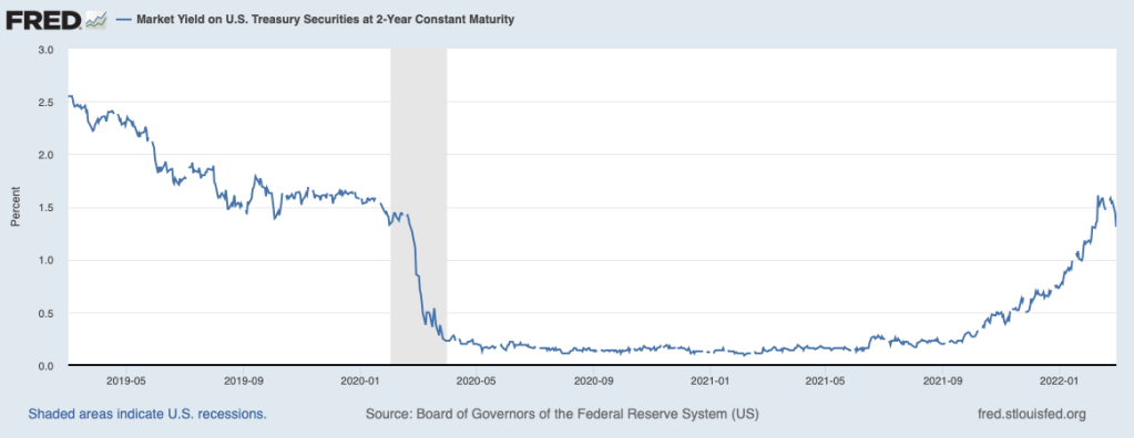
On March 2, 2022, as the conflict between Russia and Ukraine intensified, an article in the Wall Street Journal had the headline “Investors Pile Into Treasurys as Growth Concerns Flare.” The article noted that: “The 10-year Treasury yield just recorded its largest two-day decline since March 2020, while two-year Treasury yields plunged the most since 2008.”
a. What does it mean for investors to “pile into” Treasury bonds?
b. Why would investors piling into Treasury bonds cause their yields to fall?
c. What are “growth concerns”? What kind of growth are investors concerned about?
d. Why might growth concerns cause investors to buy Treasury bonds?
Solving the Problem
Step 1: Review the chapter material. This problem is about the effects of slowing economic growth on interest rates, so you may want to review Chapter 10, Section 10.5, “Saving, Investment and the Financial System.” You may also want to review Chapter 6, Appendix A (in Economics, Chapter 8, Appendix A), which explains the inverse relationship between bond prices and interest rates.
Step 2: Answer part a. by explaining what the article meant by the phrase “pile into” Treasury bonds. The article is using a slang phrase that means that investors are buying a lot of Treasury bonds.
Step 3: Answer part b. by explaining why investors piling into Treasury bonds will cause the yields on the bonds to fall. As the Appendix to Chapter 6 explains, the price of a bond represents the present value of the payments that an investor will receive over the life of the bond. Lower interest rates result in a higher present value of the payments received and, therefore, higher bond prices or—which is restating the same point—higher bond prices result in lower interest rates. If investors are increasing their demand for Treasury bonds, the increased demand will cause the prices of the bonds to increase and cause the yields—or the interest rates—on the bonds to fall.
Step 4: Answer part c. by explaining the phrase “growth concerns.” In this context, the growth being discussed is economic growth—changes in real GDP. The headline indicates that investors were concerned that the Russian invasion of Ukraine might lead to slower economic growth in the United States.
Step 5: Answer part d. by explaining why investors might purchase Treasury bonds if they were concerned about economic growth slowing. Using the model of the loanable funds markets discussed in Chapter 10, Section 10.5, we know that if economic growth slows, firms are likely to engage in fewer new investment projects, which would shift the demand curve for loanable funds to the left and result in a lower equilibrium interest rate. Investors who have purchased Treasury bonds will gain from a lower interest rate because the price of the Treasury bonds they own will increase. In addition, stock prices depend on investors’ expectations of the future profitability of firms issuing the stock. Typically, if investors believe that economic growth is likely to be slower in the future than they had previously expected, stock prices will fall, which would make Treasury bonds a more attractive investment. Finally, investors believe there is no chance that the U.S. Treasury will default on its bonds by not making the interest payments on the bonds. During an economic slowdown, investors may come to believe that the default risk on corporate bonds has increased because some corporations may run into financial problems. An increase in the default risk on corporate bonds increases the relative attractiveness of Treasury bonds as an investment.
Source: Gunjan Banerji, “Investors Pile Into Treasurys as Growth Concerns Flare,” Wall Street Journal, March 2, 2022.
Authors Glenn Hubbard & Tony O’Brien reflect on the global economic effects of Russia’s invasion of Ukraine last week. They consider the impact on the global commodity market, US monetary policy, and the impact on the financial markets in the US. Impact touches Introductory Economics, Money & Banking, International Economics, and Intermediate Macroeconomics as the effects of Russia’s aggression moves into its second week.
A map of Europe with Ukraine in the middle right below Belarus and to the east of Poland.
On Tuesday, March 1, Glenn and Tony will record a podcast on the economic consequences of the Russian invasion of Ukraine. The recording will be posted to this blog and also available through iTunes.
Some useful links
General information on developments (political and military, as well as economic):
Updates on the website of the Financial Times (note that the FT has dropped its paywall to allow non-subscribers to read this content). This article on the possible effects on the global economy is particularly worth reading.
The Twitter feed of Max Seddon, the FT’s Moscow bureau chief, is here.
The website of the New York Times has an extensive series of updates focused on military and political developments (subscription may be required).
Streaming updates on the website of the Wall Street Journal (subscription may be required).
A Twitter feed that provides timely updates on the military situation.
An article in the New Yorker discussing Russian President Vladimir Putin’s claims about the historical relationship between Russia and Ukraine.
A pessimistic blog post by a retired U.S. Army Colonel on whether the U.S. military is equipped to fight a war in Europe.
Discussions focused on economics:
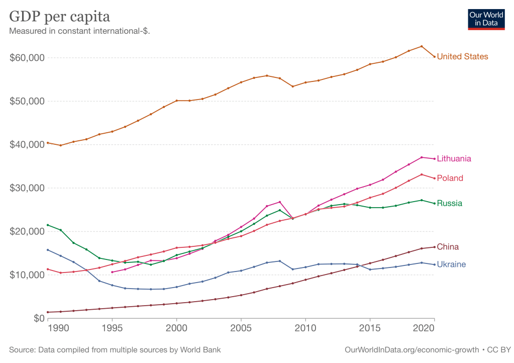
As background, the following figure from the Our World in Data site shows the growth in real GDP per capita for several countries. The underlying data were compiled by the World Bank and are measured in constant international dollars, which means that they are corrected for inflation and for variations across countries in the purchasing power of the domestic currency.
In 2020, Russian GDP per capita was less than half that of U.S. GDP per capita although about 50 percent greater than GDP per capita in China. GDP per capita in Lithuania, part of the Soviet Union until 1991, and Poland, part of the Soviet bloc until 1989, are significantly higher than in Russia. These two countries have become integrated into the European economy and have grown more rapidly than has Russia, which continues to rely heavy on exports of oil, natural gas, and other commodities. Ukraine is not as well integrated into the European economy as are Poland and Lithuania and Ukraine experienced little economic growth since attaining independence in 1991. In fact, Ukraine’s real GDP per capita was lower in 2020 than it had been in 1991.
Here is a transcript of President Joe Biden’s speech imposing sanctions on Russia.
Informative Full Stack Economics blog post by Alan Cole explaining the likely reasons why U.S. and European sanctions on Russia excluded energy. Useful explanation of the role of correspondent banking in international trade.
An article in the Economist discussing sanctions (subscription may be required).
An article in the New York Times discussing the SWIFT (Society for Worldwide Interbank Financial Telecommunications) service, which is based in Belgium, and is a key component of the international financial system. Some policymakers have proposed cutting Russia off from SWIFT. The article discusses why some countries have been opposed to taking that step (subscription may be required).
An opinion column by Justin Fox on bloomberg.com examines in what sense the United States is energy independent and the economic reasons that the U.S. still imports some oil from Russia (subscription may be required).
Blog post by economic writer Noah Smith on the possible effects of the invasion on the post-World War II international economic system.
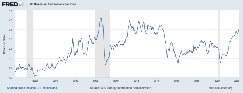
The federal government levies an excise tax of 18.4 cents per gallon of gasoline. (An excise tax is a tax that a government imposes on a particular product. In addition to the tax on gasoline, the federal government imposes excise taxes on tobacco, alcohol, airline tickets, and a few other products.) In February 2022, inflation was running at the highest level in several decades. The average retail price of gasoline across the country had risen to $3.50 per gallon from $2.60 per gallon a year earlier. The following figure shows fluctuations in the retail price of gasoline since January 2000.
Policymakers were looking for ways to lessen the effects of inflation on consumers. An article in the Wall Street Journalreported that several Democratic members of the U.S. Senate, including Mark Kelly of Arizona, Maggie Hassan of New Hampshire, and Raphael Warnock of Georgia proposed that the federal excise tax on gasoline be suspended for the remainder of 2022. The sponsors of the proposal believed that cutting the tax would reduce the price of gasoline that consumers pay at the pump. Other members of the Senate weren’t so sure, with one quoted as saying that cutting the tax was “not going to change anything” and another arguing that oil companies would receive most of the benefit of the tax cut.
Some members of Congress were opposed to suspending the gasoline tax because the revenue raised from the tax is placed in the highway trust fund, which helps to pay for federal contributions to highway building and repair and for mass transit. In that sense, the gasoline tax follows the benefits-received principle, under which people who receive benefits from a government program—in this case, highway maintenance—should help pay for the program. (We discuss the principles for evaluating taxes in Microeconomics, Chapter 17, Section 17.2 and in Economics, Chapter 17, Section 17.2) Other members of Congress were opposed to suspending the tax because they believe that the tax helps to reduce the quantity of gasoline consumed, thereby helping to slow climate change.
Focusing just on the question of the effect of suspending the tax on the retail price of gasoline, what can we conclude? The question is one of tax incidence, which looks at the actual division of the burden of a tax between buyers and sellers in a market. In other words, tax incidence looks beyond the fact that gasoline stations collect the tax and send the revenue to federal government to the issue of who actually pays the tax. As we note in Chapter 17, Section 17.3:
When the demand for a product is less elastic than supply, consumers pay the majority of the tax on the product. When the demand for a product is more elastic than supply, firms pay the majority of the tax on the product.
Consumers would receive all of the tax cut—that is, the retail price of gasoline would fall by 18.4 cents—only in the polar case where the demand for gasoline were perfectly price inelastic. Similarly, consumers would receive none of the tax cut and the price of gasoline would remain unchanged—so oil companies would receive all of the tax cut—only in the polar case where the demand for gasoline is perfectly price inelastic. (It’s a worthwhile exercise to show these two cases using demand and supply graphs.)
In the real world, we would expect to be somewhere in between these two cases, with consumers receiving some of the benefit of suspending the tax and producers receiving the remainder of the benefit. The short-run price elasticity of demand for gasoline is quite small; according to one estimate it is only −.06. The short-run price elasticity of supply of gasoline is likely to be somewhat larger than that in absolute value, which means that we would expect that consumers would receive the majority of the tax cut. (Note that we would expect the long-run price elasticities of demand and supply to both be larger for reasons we discuss in Chapter 6, Section 6.2 and 6.6.) In other words, the retail price of gasoline would fall, holding all other factors constant, but not by the full tax cut of 18.4 cents.
Joseph Doyle of MIT and Krislert Samphantharak of the University of California, San Diego studied the effect of suspension in the state excise tax on gasoline in Indiana and Illinois in 2000. In that year, Indiana suspended collecting its gasoline excise tax for 120 days and Illinois suspended its tax for 184 days. The authors estimate that consumers received about 70 percent of the tax cut in the form of lower gasoline prices. If we apply that estimate to the federal gasoline tax, then suspending the tax would lower the price of gasoline by about 12.9 cents per gallon, holding all other factors that affect the price of gasoline constant. As the above figure shows, the retail price of gasoline frequently fluctuates up and down by more than 12.9 cents, even over fairly brief periods of time. In that sense, the effect on the gasoline market of suspending the federal excise tax on gasoline would be relatively small.
Sources: Andrew Duehren and Richard Rubin, “Some Lawmakers Want to Halt Gas Tax Amid High Inflation. Others See a Gimmick,” Wall Street Journal, February 16, 2022; Tony Romm and Jeff Stein, “White House, Congressional Democrats Eye Pause of Federal Gas Tax as Prices Remain High, Election Looms,” Washington Post, February 15, 2022; Joseph J. Doyle, Jr., Krislert Samphantharak, “$2.00 Gas! Studying the Effects of a Gas Tax Moratorium,” Journal of Public Economics, Vol. 92, No.s 3-4, April 2008, pp. 869-884; and Federal Reserve Bank of St. Louis.
Cecilia Rouse, chair of the Council of Economic Advisers. Photo from the Washington Post.
An article in the Washington Post discussed a debate among President Biden’s economic advisers. The debate was over “over whether the White House should blame corporate consolidation and monopoly power for price hikes.” Some members of the National Economic Council supported the view that the increase in inflation that began in the spring of 2021 was the result of a decline in competition in the U.S. economy.
Some Democratic members of Congress have also supported this view. For instance, Massachusetts Senator Elizabeth Warren argued on Twitter that: “One clear explanation for higher inflation? Giant corporations are exploiting their market power to further raise prices. And corporate executives are bragging about their higher profits.” Or, as Vermont Senator Bernie Sanders put it: “The problem is not inflation. The problem is corporate greed, collusion & profiteering.”
But according to the article, Cecilia Rouse, chair of the President’s Council of Economic Advisers (CEA), and other members of the CEA are skeptical that a lack of competition are the main reason for the increase in inflation, arguing that very expansionary monetary and fiscal policies, along with disruptions to supply chains, have been more important.
In an earlier blog post (found here), we noted that a large majority of more than 40 well-known academic economists surveyed by the Booth School of Business at the University of Chicago disagreed with the statement: “A significant factor behind today’s higher US inflation is dominant corporations in uncompetitive markets taking advantage of their market power to raise prices in order to increase their profit margins.”
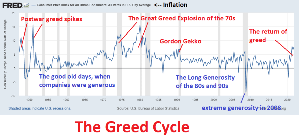
One difficulty with the argument that the sharp increase in inflation since mid-2021 was due to corporate greed is that there is no particular reason to believe that corporations suddenly became more greedy than they had been when inflation was much lower. If inflation were mainly due to corporate greed, then greed must fluctuate over time, just as inflation does. Economic writer and blogger Noah Smith poked fun at this idea in the following graph.
It’s worth noting that “greed” is one way of characterizing the self-interested behavior that underlies the assumption that firms maximize profits and individual maximize utility. (We discuss profit maximization in Microeconomics, Chapter 12, Section 12.2, and utility maximization in Chapter 10, Section 10.1.) When economists discuss self-interested behavior, they are not making a normative statement that it’s good for people to be self-interested. Instead, they are making a positive statement that economic models that assume that businesses maximize profit and consumers maximize utility have been successful in analyzing and predicting the behavior of businesses and households.
Corporate profits increased from $1.95 trillion in the first quarter of 2021 to $2.40 trillion in third quarter of 2021 (the most recent quarter for which data are available). Using another measure of profit, during the same period, corporate profits increased from about 16 percent of value added by nonfinancial corporate businesses to about 18 percent. (Value added measures the market value a firm adds to a product. We discuss calculating value added in Macroeconomics, Chapter 8, Section 8.1.)
There have been mergers in some industries that may have contributed to an increase in profits—the Biden Administration has singled out mergers in the meatpacking industry as having led to higher beef and chicken prices. At this point, though, it’s not possible to gauge the extent to which mergers have been responsible for higher prices, even in the meatpacking industry.
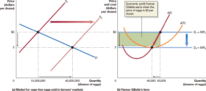
An increase in profit is not by itself an indication that firms have increased their market power. We would expect that even in a perfectly competitive industry, an increase in demand will lead in the short run to an increase in the economic profit earned by firms in the industry. But in the long run we expect economic profit to be competed away either by existing firms expanding their production or by new firms entering the industry.
In Chapter 12, we use Figure 12.8 to illustrate the effects of entry in the market for cage-free eggs. Panel (a) shows the market for cage-free eggs, made up of all the egg sellers and egg buyers. Panel (b) shows the situation facing one farmer producing cage-free eggs. (Note the very different scales of the horizontal axes in the two panels.) At $3 per dozen eggs, the typical egg farmer is earning an economic profit, shown by the green rectangle in panel (b). That economic profit attracts new entrants to the market—perhaps, in this case, egg farmers who convert to using cage-free methods. The result of entry is a movement down the demand curve to a new equilibrium price of $2 per dozen. At that price, the typical egg farmer is no longer earning an economic profit.
A few last observations:
The recent increase in profits may also be short-lived if it reflects a temporary increase in demand for some durable goods, such as furniture and appliances, raising their prices and increasing the profits of firms that produce them. The increase in spending on goods, and reduced spending on services, appears to have resulted from: (1) Households having additional funds to spend as a result of the payments they received from fiscal policy actions in 2020 and early 2021, and (2) a reluctance of households to spend on some services, such as restaurant meals and movie theater tickets, due to the effects of the Covid-19 pandemic.
The increase in profits in some industries may also be due to a reduction in supply in those industries having forced up prices. For instance, a shortage of semiconductors has reduced the supply of automobiles, raising car prices and the profits of automobile manufacturers. Over time, supply in these industries should increase, bringing down both prices and profits.
If some changes in consumer demand persist over time, we would expect that the economic profits firms are earning in the affected industries will attract the entry of new firms—a process we illustrated above. In early 2022, this process is far from complete because it takes time for new firms to enter an industry.
Source: Jeff Stein, “White House economists push back against pressure to blame corporations for inflation,” Washington Post, February 17, 2022; Mike Dorning, “Biden Launches Plan to Fight Meatpacker Giants on Inflation,” bloomberg.com, January 3, 2022; and U.S. Bureau of Economic Analysis.ec
There’s a consensus among economists that increases in unemployment during a recession typically are larger for lower-income people than for higher-income people. Lower-income people are more likely to hold jobs requiring fewer skills and firms typically expect that when they lay off less-skilled workers during a recession they will be able to higher them—or other workers with similar skills—back after the recession ends. Because higher income have skills that may be difficult to replace, firms are more reluctant to lay them off.
For instance, in an earlier blog post (found here) we noted that during the period in 2020 when many restaurants were closed, the Cheesecake Factory continued to pay its 3,000 managers while it laid off most of its servers. That strategy made it easier for the restaurant chain to more easily expand its operations when the worst of government-ordered closures were over. More generally, Serdar Birinci and YiLi Chien of the Federal Reserve Bank of St. Louis found that workers in the lowest 20 percent (or quintile) of earnings experienced an increased unemployment rate from 4.4 percent in January 2020 to 23.4 percent in April 2020, whereas workers in the highest quintile of earnings experienced an increase only from 1.1 percent in January to 4.8 percent in April.
If lower-income people are hit harder by unemployment, are they also hit harder by inflation? Answering that question is difficult because the U.S. Bureau of Labor Statistics (BLS) doesn’t routinely release data on inflation in the prices of goods and services purchased by households at different income levels. The main measure of consumer price inflation compiled by the BLS represents changes in the consumer price index (CPI). The CPI is an index of the prices in a market basket of goods and services purchased by households living in urban areas. The information on consumer purchases comes from interviews the BLS conducts every three months with a sample of consumers and from weekly diaries in which a sample of consumers report their purchases. (We discuss the CPI in Macroeconomics, Chapter 9, Section 9.4 and in Economics, Chapter 19, Section 19.4.)
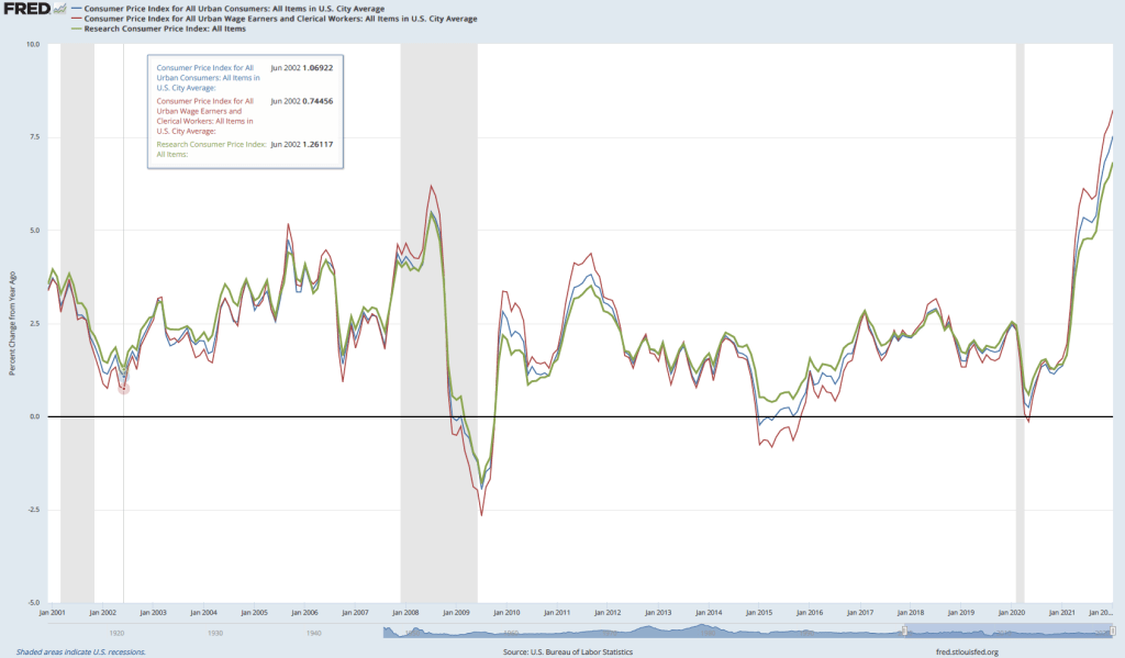
The BLS releases three measures of the CPI, the two most widely used of which are the CPI-U for all urban consumers and CPI-W for urban wage earners. CPI-W covers the subset of households that receive at least half their household income from clerical or wage occupations and who have at least one wage earner who worked for 37 weeks or more during the previous year. CPI-U represents about 93 percent of the U.S. population and CPI-W represents about 29 percent of the U.S. population. Finally, in 1988 Congress instructed the BLS to compile a consumer price index reflecting the purchases of people aged 62 and older. This version of the CPI is labeled R-CPI-E; the R indicates that it is a research series and the E indicates that it is intended to measure the prices of goods and services purchased by elderly people. Because the sample used to calculate the R-CPI-E is relatively small and because of some other difficulties that may reduce the accuracy of the index, the BLS considers it a series best suited for research and does not include the data in its monthly “Consumer Price Index” publication. In any event, as the following figure shows, inflation, measured as the percentage change in the CPI from the same month in the previous year, has been very similar for all three measures of the CPI.
Because the market baskets of goods and services consumed by a mix of high and low-income households is included in all three versions of the CPI, none of the versions provides a way to measure the possibly different effects of inflation on low-income and on high-income households. A study by Josh Klick and Anya Stockburger of the BLS attempts to fill this gap by constructing measures of the CPI for low-income and for high-income households. They define low-income households as those in the bottom 25 percent (quartile) of the income distribution and high-income households as those in the top quartile of the income distribution. During the time period of their analysis—December 2003 to December 2018—the bottom quartile had average annual incomes of $12,705 and the top quartile had average annual incomes of $155,045.
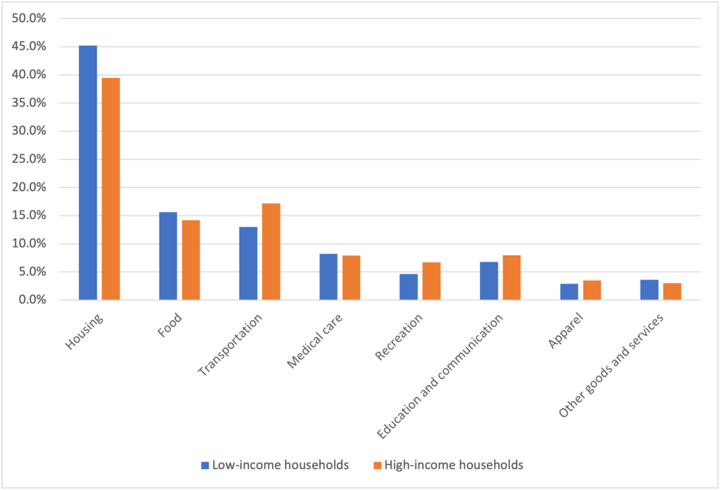
The BLS researchers constructed market baskets for the two groups. The expenditure weights—representing the mix of products purchased—don’t differ too strikingly between lower-income and higher-income households, as the figure below shows. The largest differences are housing, with low-income households having a market basket weight of 45.2 percent and high-income households having a market basket weight of 39.5 percent, and transportation, with low-income households having a market basket weight of 13.0 percent and high-income households having a market basket weight of 17.2 percent.
The following table shows the inflation rate as measured by changes in different versions of the CPI over the period from December 2003 to December 2018. During this period, the CPI-U (the version of the CPI that is most frequently quoted in news stories) increased at an annual rate of 2.1 percent, which was the same rate as the CPI-W. The R-CPI-E increased at a slightly faster rate of 2.2 percent. Lower-income households experienced the highest inflation rate at 2.3 percent and higher-income households experienced the lowest inflation rate of 2.0 percent.
CPI-U
CPI-W
R-CPI-E
CPI for lowest income quartile
CPI for highest income quartile
2.1%
2.2%
2.1%
2.3%
2.0%
The differences in inflation rates across groups were fairly small. Can we conclude that the same was true during the recent period of much higher inflation rates? We won’t know with certainty until the BLS extends its analysis to cover at least the years 2021 and 2022. But we can make a couple of relevant observations. First, for many people the most important aspect of inflation is whether prices are increasing faster of slower than their wages. In other words, people are interested in what is happening to their real wage. (We discuss calculating real wage rates in Macroeconomics, Chapter 9, Section 9.5 and in Economics, Chapter 19, Section 19.5.)
The Federal Reserve Bank of Atlanta compiles data on wage growth, including wage growth by workers in different income quartiles. The following figure shows that workers in the top quartile have experienced more rapid wage growth in the months since the beginning of the Covid-19 pandemic than have workers in the other quartiles. This gap continues a trend that began in 2015. The bottom quartile has experienced the slowest rate of income growth. (Note that the researchers at the Atlanta Fed compute wage growth as a 12-month moving average rather than as the percentage from the same month in the previous year, as we have been doing when calculating inflation using the CPI.) For example, in January 2022, calculated this way, average wage growth in the top quartile was 5.8 percent as opposed to 2.9 percent in the bottom quartile.
As with any average, there is some variation in the experiences of different individuals. Although, as a group, lower-income workers have seen wage growth that lags behind other workers, in some industries that employ many lower-income people, wage growth has been strong. For instance, as measured by average hourly earnings, wages for all workers in the private sector increased by 5.7 percent between January 2021 and 2022. But average hourly earnings in the leisure and hospitality industry—which employs many lower-income workers—increased by 13.0 percent.
Overall, it seems likely that the real wages of higher-income workers have been increasing while the real wages of lower-income workers have been decreasing, although the experience of individual workers in both groups may be very different than the average experience.
Sources: Josh Klick and Anya Stockburger, “Experimental CPI for Lower and Higher Income Households Serdar,” U.S. Bureau of Labor Statistics, Working Paper 537, March 8, 2021; Birinci and YiLi Chien, “An Uneven Crisis for Lower-Income Households,” Federal Reserve Bank of St. Louis, Annual Report 2020, April 7, 2021; and Federal Reserve Bank of Atlanta, “Wage Growth Tracker,” https://www.atlantafed.org/chcs/wage-growth-tracker.
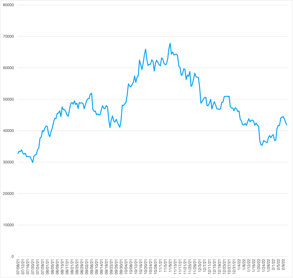
Bitcoin has failed in their original purpose of providing a digital currency that could be used in everyday transactions like buying lunch and paying a cellphone bill. As the following figure shows, swings in the value of bitcoin have been too large to make useful as a medium of exchange like dollar bills. During the period shown in the figure—from July 2021 to February 2022—the price of bitcoin has increased by more than $30,000 per bitcoin and then fallen by about the same amount. Bitcoin has become a speculative asset like gold. (We discuss bitcoin in the Apply the Concept, “Are Bitcoins Money?” which appears in Macroeconomics, Chapter 14, Section 14.2 and in Economics, Chapter 24, Section 24.2. In an earlier blog post found here we discussed how bitcoin has become similar to gold.)
The vertical axis measures the price of bitcoin in dollars per bitcoin.
The Slow U.S. Payments Increases the Appeal of a Digital Currency
Some economists and policymakers argue that there is a need for a digital currency that would do what bitcoin was originally intended to do—serve as a medium of exchange. Digital currencies hold the promise of providing a real-time payments system, which allow payments, such as bank checks, to be made available instantly. The banking systems of other countries, including Japan, China, Mexico, and many European countries, have real-time payment systems in which checks and other payments are cleared and funds made available in a few minutes or less. In contrast, in the United States, it can two days or longer after you deposit a check for the funds to be made available in your account.
The failure of the United States to adopt a real-time payments system has been costly to many lower-income people who are likely to need paychecks and other payments to be quickly available. In practice, many lower-income people: 1) incur bank overdraft fees, when they write checks in excess of the funds available in their accounts, 2) borrow money at high interest rates from payday lenders, or 3) pay a fee to a check cashing store when they need money more quickly than a bank will clear a check. Aaron Klein of the Brookings Institution estimates that lower-income people in the United States spend $34 billion annually as a result of relying on these sources of funds. (We discuss the U.S. payments system in Money, Banking, and the Financial System, 4th edition, Chapter 2, Section 2.3.)
The Problem with Stablecoins as Money
Some entrepreneurs have tried to return to the original idea of using cryptocurrencies as a medium of exchange by introducing stablecoins that can be bought and sold for a constant number of dollars—typically one dollar for one stablecoin. The issuers of stablecoins hold in reserve dollars, or very liquid assets like U.S. Treasury bills, to make credible the claim that holders of stablecoins will be able to exchange them one-for-one for dollars. Tether and Circle Internet Financial are the leading issuers of stablecoins.
So far, stablecoins have been used primarily to buy bitcoin and other cryptocurrencies rather than for day-to-day buying and selling of goods and services in stores or online. Financial regulators, including the U.S. Treasury and the Federal Reserve, are concerned that stablecoins could be a risk to the financial system. These regulators worry that issuers of stablecoins may not, in fact, keep sufficient assets in reserve to redeem them. As a result, stablecoins might be susceptible to runs similar to those that plagued the commercial banking system prior to the establishment of the Federal Deposit Insurance Corporation in the 1930s or that were experienced by some financial firms during the 2008 financial crisis. In a run, issuers of stablecoins might have to sell financial assets, such as Treasury bills, to be able to redeem the stablecoins they have issued. The result could be a sharp decline in the prices of these assets, which would reduce the financial strength of other firms holding the assets.
In 2019, Facebook (whose corporate name is now Meta Platforms) along with several other firms, including PayPal and credit card firm Visa, began preparations to launch a stablecoin named Libra—the name was later changed to Diem. In May 2021, the firms backing Diem announced that Silvergate Bank, a commercial bank in California, would issue the Diem stablecoin. But according to an article in the Wall Street Journal, the Federal Reserve had “concerns about [the stablecoin’s] effect on financial stability and data privacy and worried [it] could be misused by money launderers and terrorist financiers.” In early 2022, Diem sold its intellectual property to Silvergate, which hoped to still issue the stablecoin at some point.
A Federal Reserve Digital Currency?
If private firms or individual commercial banks have not yet been able to issue a digital currency that can be used in regular buying and selling in stores and online, should central banks do so? In January 2022, the Federal Reserve issued a report discussing the issues involved with a central bank digital currency (CBCD). As we discuss in Macroeconomics, Chapter 14, Section 14.2, most of the money supply of the United States consists of bank deposits. As the Fed’s report points out, because bank deposits are computer entries on banks’ balance sheets, most of the money in the United States today is already digital. As we discuss in Section 14.3, bank deposits are liabilities of commercial banks. In contrast, a CBCD would be a liability of the Fed or other central bank.
The Fed report lists the benefits of a CBCD:
“[I]t could provide households and businesses [with] a convenient, electronic form of central bank money, with the safety and liquidity that would entail; give entrepreneurs a platform on which to create new financial products and services; support faster and cheaper payments (including cross-border payments); and expand consumer access to the financial system.”
Importantly, the Fed indicates that it won’t begin issuing a CBCD without the backing of the president and Congress: “The Federal Reserve does not intend to proceed with issuance of a CBDC without clear support from the executive branch and from Congress, ideally in the form of a specific authorizing law.”
The Fed report acknowledges that “a significant number of Americans currently lack access to digital banking and payment services. Additionally, some payments—especially cross-border payments—remain slow and costly.” By issuing a CBDC, the Fed could help to reduce these problems by making digital banking services available to nearly everyone, including lower-income people who currently lack bank checking accounts, and by allowing consumers to have payments instantly available rather than having to wait for a check to clear.
The report notes that: “A CBDC would be the safest digital asset available to the general public, with no associated credit or liquidity risk.” Credit risk is the risk that the value of the currency might decline. Because the Fed would be willing to redeem a dollar of CBDC currency for a dollar or paper money, a CBDC has no credit risk. Liquidity risk is the risk that, particularly during a financial crisis, someone holding CBDC might not be able to use it to buy goods and services or financial assets. Fed backing of the CBDC makes it unlikely that someone holding CBDC would have difficulty using it to buy goods and services or financial assets.
But the report also notes several risks that may result from the Fed issuing a CBDC:
Banks rely on deposits for the funds they use to make loans to households and firms. If large numbers of households and firms switch from using checking accounts to using CBDC, banks will lose deposits and may have difficulty funding loans.
If the Fed pays interest on the CBDC it issues, households, firms, and investors may switch funds from Treasury bills, money market mutual funds, and other short-term assets to the CBDC, which might potentially disrupt the financial system. Money market mutual funds buy significant amounts of corporate commercial paper. Some corporations rely heavily on the funds they raise from selling commercial paper to fund their short-term credit needs, including paying suppliers and financial inventories.
In a financial panic, many people may withdraw funds from commercial bank deposits and convert the funds into CBDC. These actions might destabilize the banking system.
A related point: A CBDC might result in large swings in bank reserves, particularly during and after a financial panic. As we discuss in Macroeconomics, Chapter 14, Section 14.4 (Economics, Chapter 24, Section 24.4), increasing and decreasing bank reserves is one way in which the Fed carries out monetary policy. So fluctuations in bank reserves may make it more difficult for the Fed to conduct monetary policy, particularly during a financial panic. (This consideration is less important during times like the present when banks hold very large reserves.)
Because the Fed has no experience in operating a retail banking operation, it would be likely that if it began issuing a CBDC, it would do so through commercial banks or other financial firms rather than doing so directly. These financial firms would then hold customers CBDC accounts and carry out the actual flow of payments in CBDC among households and firms.
The report notes that the Fed is only beginning to consider the many issues that would be involved in issuing a CBDC and still needs to gather feedback from the general public, financial firms, nonfinancial firms, and investors, as well as from policymakers in Washington.
Sources: Peter Rudegeair and Liz Hoffman, “Facebook’s Cryptocurrency Venture to Wind Down, Sell Assets,” Wall Street Journal, January 26, 2022; Liana Baker, Jesse Hamilton, and Olga Kharif, “Mark Zuckerberg’s Stablecoin Ambitions Unravel with Diem Sale Talks,” bloomberg.com, January 25, 2022; Amara Omeokwe, “U.S. Regulators Raise Concern With Stablecoin Digital Currency,” Wall Street Journal, December 17, 2022; Jeanna Smialek, “Fed Opens Debate over a U.S. Central Bank Digital Currency with Long-Awaited Report,”, January 20, 2022; Board of Governors of the Federal Reserve System, Money and Payments: The U.S. Dollar in the Age of Digital Transformation, January 2022; and Aaron Klein, “The Fastest Way to Address Income Inequality? Implement a Real Time Payments System,” brookings.edu, January 2, 2019.
An article in the Wall Street Journal quoted an economist at a financial services firm as noting that strong growth in wages could lead to sustained inflation. The article stated that as a result “the yield on the 10-year U.S. Treasury note [rose to] within reach of 2%” and that: “Rising [bond] yields this year have rattled markets and hurt tech stocks in particular ….”
What are the links between wage inflation and price inflation, inflation and bond yields, and bond yields and stock prices—particularly the prices of tech stocks?
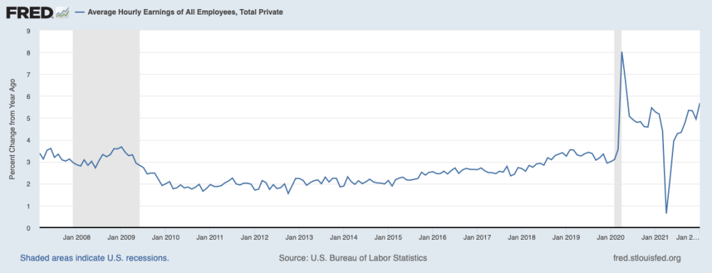
The link between wage inflation and price inflation. The monthly “Employment Situation” reports from the Bureau of Labor Statistics (BLS), in addition to providing data on payroll employment and the unemployment rate, also provide data on average hourly earnings (AHE). AHE are the wages and salaries per hour worked that private, nonfarm business pay workers. AHE don’t include the value of benefits that firms provide workers, such as contributions to 401(k) retirement accounts or health insurance. The following figure shows changes in AHE from the same month in the previous year. The figure shows that since the Covid-19 pandemic first began to affect the U.S. economy in March 2020, AHE have moved erratically. But since the fall of 2021, growth in AHE has been consistently above the 2 percent to 4 percent range that prevailed in the years after the end of the Great Recession of 2007–2009.
Employee compensation is the largest cost for most firms. For the economy as whole, employee compensation is about 80 percent of total costs. When firms pay higher wages per hour, their costs per unit of output don’t rise unless the wage increases are greater than the rate of growth of labor productivity, or output per hour worked. Increases in wages in the range of 5 percent to 6 percent are well above the rate of growth of labor productivity and, so, firms are likely to pass through the wage increases by raising prices. Note that the higher prices may prompt workers to push for higher wage increases to offset the decline in the real purchasing power of their wages, potentially setting off a wage-price spiral. (We discussed the possibility of a wage-price spiral in a recent post here.)
The link between inflation and bond yields. When investors lend money by, for instance, buying a bond, they are concerned with the interest rate they will receive after correcting for the effects of inflation. In other words, they focus on the real interest rate, which is equal to the nominal interest rate, or the stated interest rate on the loan or bond, minus the expected inflation rate:
The second equation indicates that if investors expect the inflation rate to increase, then, unless the real interest rate changes, the nominal interest rate will increase. The Fisher effect is the idea associated with Yale economist Irving Fisher that the nominal interest rate rises or falls by the same number of percentage points as the expected inflation rate. So, for instance, if investors expect that the inflation rate will increase from 3 percent to 5 percent, then the nominal interest rate will also increase by two percentage points.
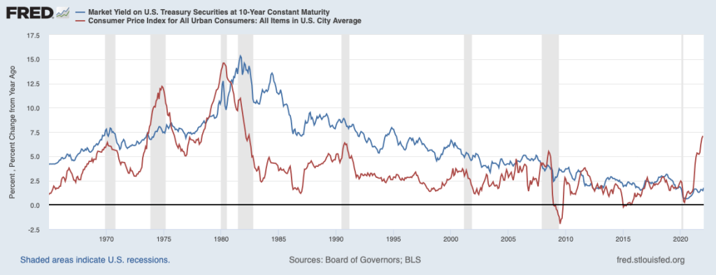
Because of real-world frictions, such as the broker fees that investors pay when buying and selling bonds and the taxes investors pay when they sell a bond that has increased in price, the Fisher effect doesn’t hold exactly. Still, most economists agree that an increase in the expected inflation rate will cause an increase in nominal interest rates. The following figure shows movements in the interest rate on 10-year Treasury notes (blue line) and in inflation (red line). Note that, roughly speaking, the interest rate on the 10-year Treasury note is higher when inflation is higher and lower when inflation is lower. (We discuss real and nominal interest rates in Macroeconomics, Chapter 9, Section 9.6 and in Economics, Chapter 19, Section 19.6. We discuss the Fisher effect in Money, Banking, and the Financial System, Chapter 4, Section 4.3.)
The link between bond yields and stock prices. As wage inflation leads to price inflation and price inflation leads to higher interest rates on bonds—particularly U.S. Treasury bonds—why might stock prices be affected? First, investors consider U.S. Treasury bonds to be default risk free, which means that investors are certain that the Treasury will make the interest and principal payments on the bonds. Stock investments are much riskier because they depend on the future profits of the firms issuing the stocks and those profits may fluctuate in ways that are difficult for investors to anticipate. So as interest rates on Treasury bonds increase, some investors will decide to sell stocks and buy bonds, which will cause a decline in stock prices.
Second, most people value funds they will receive now or soon more highly than funds they will receive in the more distant future. For instance, if someone offered to pay you $1,000 today or $1,000 one year from now, you will prefer to receive the money today. In other words, the present value, or value today, of a payment you won’t receive until the future is worth less than the face value of the payment. For instance, the present value of $1,000 you won’t receive for a year is worth less than $1,000 in present value. The higher the interest rate is, the lower the present value of payments, such as dividends, that you will receive in the future.
Economists believe that price of a financial investment, like a bond or a stock, is equal to the present value of the payments you will receive from owning the asset. If you own a bond, you will receive interest payments and payment of the bond’s principal when the bond matures. If you own a stock, you will receive dividends, which are the payments that firms make to shareholders from the firms’ profits. Therefore stock prices should reflect the present value of the dividends that investors expect to receive from owning the stock. (We discuss present value and the relationship between interest rates and stock and bond prices in Macroeconomics, Chapter 6, Appendix, in Economics, Chapter 8, Appendix, and, more completely, in Money, Banking, and the Financial System, Chapter 3, Section 3.2 and Chapter 6, Section 6.2.)
The Wall Street Journal article we quoted above notes that the rising interest rate on the 10-year Treasury note was causing price declines in tech stocks in particular. The explanation is that tech firms often go through an initial period in which they may make very low profits or even suffer losses. Investors may still be willing to buy stock in tech firms because they expect the firms eventually to increase their profits and the dividends they pay. But because those profits will be earned in the future—often after a period of losses that may stretch for years—the present value of the profits and, therefore, the price of the stock depends more on the interest rate than would be true of a firm making breakfast cereal or frozen pizza that will be steadily earning profits through the years. Therefore, we would expect, as the article indicates, that the prices of tech firms are more likely to decline—or to decline more—when interest rates rise than is true of other firms.
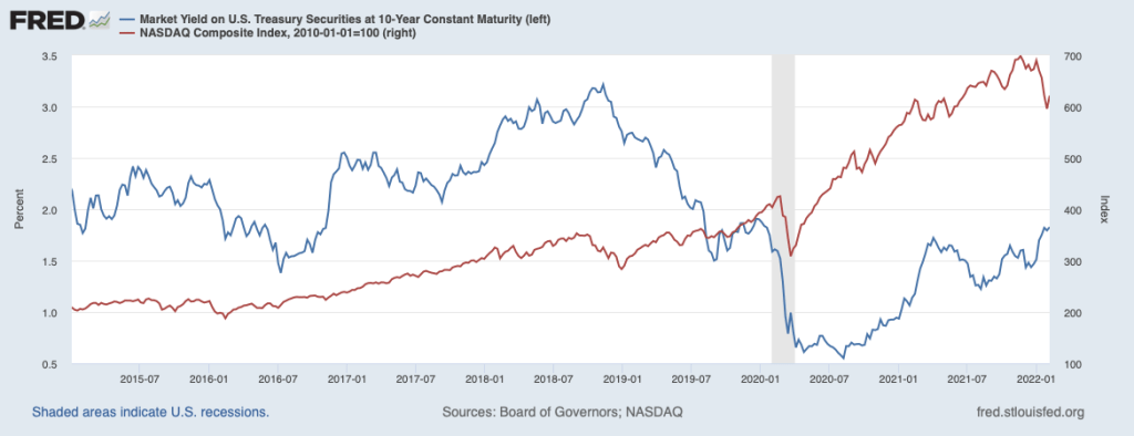
The following figure shows the interest rate on the 10-year Treasury note (blue line with scale given on the left) and the values of the Nasdaq composite stock index (red line with the value for January 1, 2010 set equal to 100 and the scale given on the right). The Nasdaq includes the stocks of more tech firms than is true of the other widely followed stock market indexes—the S&P 500 and the Dow Jones Industrial Average. The figure shows that the declining interest rate on 10-year Treasury notes that began in late 2018 and continued through mid-2020 coincided with increases in the prices of the stocks in the Nasdaq index—apart from the spring of 2020 during the beginning of the Covid-19 pandemic. The most recent period shows that increases in the interest rate on the 10-year Treasury note have corresponded with a decline in the Nasdaq, as noted in the article.
Source: Sam Goldfarb, “Elevated Bond Yields Approach Key Milestone,” Wall Street Journal, February 7, 2022; U.S. Bureau of Economic Analysis, “Prices, Costs, and Profit per Unit of Real Gross Value Added of Nonfinancial Domestic Corporate Business,” January 27, 2022; and Federal Reserve Bank of St. Louis.
On Sunday, February 6, the New York Times ran an article on Modern Monetary Theory (MMT) on the front page of its business section with the title, “Time for a Victory Lap.” Link here, subscription may be required. (Note: The title of the article was later changed on the nytimes.com site to “Is This What Winning Looks Like?” perhaps because of the controversy linked to below.)
The article led to a controversy on Twitter (but, then, what topic doesn’t lead to a controversy on Twitter?). Social media is, obviously, not always the best place to discuss economic theory and policy, but instructors and students interested in the debate may find the following links useful both because of the substantive issues raised and as an example of how debates over economic policy can sometimes become heated.
Harvard economist Lawrence Summers reacts negatively to the content of the New York Times article (and to MMT) here.
Economics blogger Noah Smith also reacts negatively to the article here. Smith’s blog post discussing the article at length is here, subscription may be required.
Former Fed economist Claudia Sahm defends the article (and MMT) here.
Jeanna Smialek, the author of the New York Times article, reacts to critics of the article here and to Noah Smith’s blog post here. Smith responds to her response here.
Jason Furman of Harvard’s Kennedy School provides a brief discussion of whether MMT has had much influence on monetary policy here.
We discuss MMT in the Apply the Concept, “Modern Monetary Theory: Should We Stop Worrying and Love the Debt?” in Macroeconomics, Chapter 16, Section 16.6 and in Economics, Chapter 26, Section 26.6.