Supports:Macroeconomics, Chapter 18, Economics, Chapter 28, and Essentials of Economics, Chapter 19.
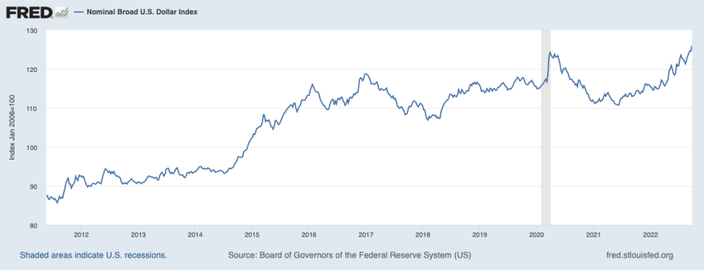
Between June 2021 and September 2022, the exchange rate between the U.S. dollar and an average of the currencies of the major trading partners of the United States increased by 14 percent. (This movement is shown in the figure above.) An article in the New York Times had the headline “The Dollar Is Strong. That Is Good for the U.S. but Bad for the World.”
Briefly explain what the headline means by a “strong” dollar.
Do you agree with the assertion in the headline that a stronger dollar is good for the United States but bad for the economies that the United States trades with? Briefly explain.
During this period the Federal Reserve was taking actions that raised U.S. interest rates. The article noted that “Those interest rate increases are pumping up the value of the dollar ….” Why would increases in U.S. interest rates relative to interest rates in other countries increase the value of the dollar?
Solving the Problem
Step 1: Review the chapter material. This problem is about the effect of fluctuations in the exchange rate and the relationship between interest rates and exchange rates, so you may want to review Macroeconomics, Chapter 18, Section 8.2, “The Foreign Exchange Market and Exchange Rates,” or the corresponding sections in Economics, Chapter 28 or Essentials of Economics, Chapter 19.
Step 2:Answer part a. by explaining what a “strong” dollar means. A strong dollar is one that exchanges for more units of foreign currencies, such as British pounds or euros. (A “weak” dollar means the opposite: A dollar that exchanges for fewer units of foreign currencies.)
Step 3: Answer part b. by explaining whether you agree with the assertion that a stronger dollar is good for the United States but bad for the economies of other countries. A stronger U.S. dollar produces winners and losers both in the United States and in other countries. U.S. consumers win because a stronger dollar means that fewer dollars are needed to buy the same quantity of a foreign currency, which reduces the dollar price of imports from that country. For example, a stronger dollar reduces the number of dollars U.S. consumers pay to buy a bottle of French wine that has a 40 euro price. A strong dollar is bad news for foreign consumers because they must pay more units of their currency to buy goods imported from the United States. For example, Japanese consumers will have to pay more yen to buy an imported Hershey’s candy bar with a $1.25 price.
The situation is reversed for U.S. and foreign firms exporting goods. Because foreign consumers have to pay higher prices in their own currencies for goods imported from the United States, they are likely to buy less of them, buying more domestically produced goods or goods imported from other countries. U.S. firms will either to have accept lower sales, or cut the prices they charge for their exports. In either case, U.S. exporters’ revenue will decline. Foreign firms that export to the United States will be in the opposite situation: The dollar prices of their exports will decline, increasing their sales.
We can conclude that the article’s headline is somewhat misleading because not all groups in the United States are helped by a strong dollar and not all groups in other countries are hurt by a strong dollar.
Step 4: Answer part c. by explaining why higher interest rates in the United States relative to interest rates in other countries will increase the exchange value of the dollar. If interest rates in the United States rise relative to interest rates in other countries—as was true during the period from the spring of 2021 to the fall of 2022—U.S. financial assets, such as U.S. Treasury bills, will be more desirable, causing investors to increase their demand for the dollars they need to buy U.S. financial assets. The resulting shift to the right in the demand curve for dollars will cause the equilibrium exchange rate between the dollar and other currencies to increase.
Source: Patricia Cohen, “The Dollar Is Strong. That Is Good for the U.S. but Bad for the World,” New York Times, September 26, 2022.
The Federal Reserve building in Washington, DC. (Photo from the Wall Street Journal.)
In the Federal Reserve Act, Congress charged the Federal Reserve with conducting monetary policy so as to achieve both “maximum employment” and “stable prices.” These two goals are referred to as the Fed’s dual mandate. (We discuss the dual mandate in Macroeconomics, Chapter 15, Section 15.1, Economics, Chapter 25, Section 25.1, and Money, Banking, and the Financial System, Chapter 15, Section 15.1.) Accordingly, when Fed chairs give their semiannual Monetary Policy Reports to Congress, they reaffirm that they are acting consistently with the dual mandate. For example, when testifying before the U.S. Senate Committee on Banking, Housing, and Urban Affairs in June 2022, Fed Chair Jerome Powell stated that: “The Fed’s monetary policy actions are guided by our mandate to promote maximum employment and stable prices for the American people.”
Despite statements of that kind, some economists argue that in practice during some periods the Fed’s policymaking Federal Open Market Committee (FOMC) acts as if it were more concerned with one of the two mandates. In particular, in the decades following the Great Inflation of the 1970s, FOMC members appear to have put more emphasis on price stability than on maximum employment. These economists argue that during these years, FOMC members were typically reluctant to pursue a monetary policy sufficiently expansionary to lead to maximum employment if the result would be to cause the inflation rate to rise above the Fed’s target of an annual target of 2 percent. (Although the Fed didn’t announce a formal inflation target of 2 percent until 2012, the FOMC agreed to set a 2 percent inflation target in 1996, although they didn’t publicly announce at the time. Implicitly, the FOMC had been acting as if it had a 2 percent target since at least the mid–1980s.)
In July 2019, the FOMC responded to a slowdown in economic growth in late 2018 and early 2019 but cutting its target for the federal funds rate. It made further cuts to the target rate in September and October 2019. These cuts helped push the unemployment rate to low levels even as the inflation rate remained below the Fed’s 2 percent target. The failure of inflation to increase despite the unemployment rate falling to low levels, provides background to the new monetary policy strategy the Fed announced in August 2020. The new monetary policy, in effect, abandoned the Fed’s previous policy of attempting to preempt a rise in the inflation rate by raising the target for the federal funds rate whenever data on unemployment and real GDP growth indicated that inflation was likely to rise. (We discussed aspects of the Fed’s new monetary policy in previous blog posts, including here, here, and here.)
In particular, the FOMC would no longer see the natural rate of unemployment as the maximum level of employment—which Congress has mandated the Fed to achieve—and, therefore, wouldn’t necessarily begin increasing its target for the federal funds rate when the unemployment rate dropped by below the natural rate. As Fed Chair Powell explained at the time, “the maximum level of employment is not directly measurable and [it] changes over time for reasons unrelated to monetary policy. The significant shifts in estimates of the natural rate of unemployment over the past decade reinforce this point.”
Many economists interpreted the Fed’s new monetary strategy and the remarks that FOMC members made concerning the strategy as an indication that the Fed had turned from focusing on the inflation rate to focusing on unemployment. Of course, given that Congress has mandated the Fed to achieve both stable prices and maximum employment, neither the Fed chair nor other members of the FOMC can state directly that they are focusing on one mandate more than the other.
The sharp acceleration in inflation that began in the spring of 2021 and continued into the fall of 2022 (shown in the following figure) has caused members of the FOMC to speak more forcefully about the need for monetary policy to bring inflation back to the Fed’s target rate of 2 percent. For example, in a speech at the Federal Reserve Bank of Kansas City’s annual monetary policy conference held in Jackson Hole, Wyoming, Fed Chair Powell spoke very directly: “The Federal Open Market Committee’s (FOMC) overarching focus right now is to bring inflation back down to our 2 percent goal.” According to an article in the Wall Street Journal, Powell had originally planned a longer speech discussing broader issues concerning monetary policy and the state of the economy—typical of the speeches that Fed chairs give at this conference—before deciding to deliver a short speech focused directly on inflation.
Members of the FOMC were concerned that a prolonged period of high inflation rates might lead workers, firms, and investors to no longer expect that the inflation rate would return to 2 percent in the near future. If the expected inflation rate were to increase, the U.S. economy might enter a wage–price spiral in which high inflation rates would lead workers to push for higher wages, which, in turn, would increase firms’ labor costs, leading them to raise prices further, in response to which workers would push for even higher wages, and so on. (We discuss the concept of a wage–price spiral in earlier blog posts here and here.)
With Powell noting in his Jackson Hole speech that the Fed would be willing to run the risk of pushing the economy into a recession if that was required to bring down the inflation rate, it seemed clear that the Fed was giving priority to its mandate for price stability over its mandate for maximum employment. An article in the Wall Street Journal quoted Richard Clarida, who served on the Fed’s Board of Governors from September 2018 until January 2022, as arguing that: “Until inflation comes down a lot, the Fed is really a single mandate central bank.”
This view was reinforced by the FOMC’s meeting on September 21, 2022 at which it raised its target for the federal funds rate by 0.75 percentage points to a range of 3 to 3.25 percent. The median projection of FOMC members was that the target rate would increase to 4.4 percent by the end of 2022, up a full percentage point from the median projection at the FOMC’s June 2022 meeting. The negative reaction of the stock market to the announcement of the FOMC’s decision is an indication that the Fed is pursuing a more contractionary monetary policy than many observers had expected. (We discuss the relationship between stock prices and economic news in this blog post.)
Some economists and policymakers have raised a broader issue concerning the Fed’s mandate: Should Congress amend the Federal Reserve Act to give the Fed the single mandate of achieving price stability? As we’ve already noted, one interpretation of the FOMC’s actions from the mid–1980s until 2019 is that it was already implicitly acting as if price stability were a more important goal than maximum employment. Or as Stanford economist John Cochrane has put it, the Fed was following “its main mandate, which is to ensure price stability.”
The main argument for the Fed having price stability as its only mandate is that most economists believe that in the long run, the Fed can affect the inflation rate but not the level of potential real GDP or the level of employment. In the long run, real GDP is equal to potential GDP, which is determined by the quantity of workers, the capital stock—including factories, office buildings, machinery and equipment, and software—and the available technology. (We discuss this point in Macroeconomics, Chapter 13, Section 13.2 and in Economics, Chapter 23, Section 23.2.) Congress and the president can use fiscal policy to affect potential GDP by, for example, changing the tax code to increase the profitability of investment, thereby increasing the capital stock, or by subsidizing apprentice programs or taking other steps to increase the labor supply. But most economists believe that the Fed lacks the tools to achieve those results.
Economists who support the idea of a single mandate argue that the Fed would be better off focusing on an economic variable they can control in the long run—the inflation rate—rather than on economic variables they can’t control—potential GDP and employment. In addition, these economists point out that some foreign central banks have a single mandate to achieve price stability. These central banks include the European Central Bank, the Bank of Japan, and the Reserve Bank of New Zealand.
Economists and policymakers who oppose having Congress revise the Federal Reserve Act to give the Fed the single mandate to achieve price stability raise several points. First, they note that monetary policy can affect the level of real GDP and employment in the short run. Particularly when the U.S. economy is in a severe recession, the Fed can speed the return to full employment by undertaking an expansionary policy. If maximum employment were no longer part of the Fed’s mandate, the FOMC might be less likely to use policy to increase the pace of economic recovery, thereby avoiding some unemployment.
Second, those opposed to the Fed having single mandate argue that the Fed was overly focused on inflation during some of the period between the mid–1980s and 2019. They argue that the result was unnecessarily low levels of employment during those years. Giving the Fed a single mandate for price stability might make periods of low employment more likely.
Finally, because over the years many members of Congress have stated that the Fed should focus more on maximum employment than price stability, in practical terms it’s unlikely that the Federal Reserve Act will be amended to give the Fed the single mandate of price stability.
In the end, the willingness of Congress to amend the Federal Reserve Act, as it has done many times since initial passage in 1914, depends on the performance of the U.S. economy and the U.S. financial system. It’s possible that if the high inflation rates of 2021–2022 were to persist into 2023 or beyond, Congress might revise the Federal Reserve Act to change the Fed’s approach to fighting inflation either by giving the Fed a single mandate for price stability or in some other way.
Sources: Board of Governors of the Federal Reserve System, “Federal Reserve Issues FOMC Statement,” federalreserve.gov, September 21, 2022; Board of Governors of the Federal Reserve System, “Summary of Economic Projections,” federalreserve.gov, September 21, 2022; Nick Timiraos, “Jerome Powell’s Inflation Whisperer: Paul Volcker,” Wall Street Journal, September 19, 2022; Matthew Boesler and Craig Torres, “Powell Talks Tough, Warning Rates Are Going to Stay High for Some Time,” bloomberg.com, August 26, 2022; Jerome H. Powell, “Semiannual Monetary Policy Report to the Congress,” June 22, 2022, federalreserve.gov; Jerome H. Powell, “Monetary Policy and Price Stability,” speech delivered at “Reassessing Constraints on the Economy and Policy,” an economic policy symposium sponsored by the Federal Reserve Bank of Kansas City, Jackson Hole, Wyoming, federalreserve.gov, August 26, 2022; John H. Cochrane, “Why Isn’t the Fed Doing its Job?” project-syndicate.org, January 19, 2022; Board of Governors of the Federal Reserve System, “Minutes of the Federal Open Market Committee Meeting on July 2–3, 1996,” federalreserve.gov; and Federal Reserve Bank of St. Louis.
On September 16, 2022 an article in the Wall Street Journal had the headline: “Economic Worries, Weak FedEx Results Push Stocks Lower.” Another article in the Wall Street Journal noted that: “The company’s downbeat forecasts, announced Thursday, intensified investors’ macroeconomic worries.”
Why would the news that FedEx had lower revenues than expected during the preceding weeks cause a decline in stock market indexes like the Dow Jones Industrial Average and the S&P 500? As the article explained: “Delivery companies [such as FedEx and its rival UPS) are the proverbial canary in the coal mine for the economy.” In other words, investors were using FedEx’s decline in revenue as a leading indicator of the business cycle. A leading indicator is an economic data series—in this case FedEx’s revenue—that starts to decline before real GDP and employment in the months before a recession and starts to increase before real GDP and employment in the months before a recession reaches a trough and turns into an expansion.
So, investors were afraid that FedEx’s falling revenue was a signal that the U.S. economy would soon enter a recession. And, in fact, FedEx CEO Raj Subramaniam was quoted as believing that the global economy would fall into a recession. As firms’ profits decline during a recession so, typically, do the prices of the firms’ stock. (As we discuss in Macroeconomics, Chapter 6, Section 6.2 and in Economics, Chapter 8, Section 8.2, stock prices reflect investors’ expectations of the future profitability of the firms issuing the stock.)
Monitoring fluctuations in FedEx’s revenue for indications of the future course of the economy is nothing new. When Alan Greenspan was chair of the Federal Reserve from 1987 to 2006, he spoke regularly with Fred Smith, the founder of FedEx and at the time CEO of the firm. Greenspan believed that changes in the number of packages FedEx shipped gave a good indication of the overall state of the economy. FedEx plays such a large role in moving packages around the country that most economists agree that there is a close relationship between fluctuations in FedEx’s business and fluctuations in GDP. Some Wall Street analysts refer to this relationship as the “FedEx Indicator” of how the economy is doing.
In September 2022, the FedEx indicator was blinking red. But the U.S. economy is complex and fluctuations in any indicator can sometimes provide an inaccurate forecast of when a recession will begin or end. And, in fact, some investment analysts believed that problems at FedEx may have been due as much to mistakes the firms’ managers had made as to general problems in the economy. As one analyst put it: “We believe a meaningful portion of FedEx’s missteps here are company-specific.”
At this point, Fed Chair Jerome Powell and the other members of the Federal Open Market Committee are still hoping that they can bring the economy in for a soft landing—bringing inflation down closer to the Fed’s 2 percent target, without bringing on a recession—despite some signals, like those being given by the FedEx indicator, that the probability of the United States entering a recession was increasing.
Sources: Will Feuer, “FedEx Stock Tumbles More Than 20% After Warning on Economic Trends,” Wall Street Journal, September 16, 2022; Alex Frangos and Hannah Miao, “ FedExt Stock Hit by Profit Warning; Rivals Also Drop Amid Recession Fears,” Wall Street Journal, September 16, 2022; Richard Clough, “FedEx has Biggest Drop in Over 40 Years After Pulling Forecast,” bloomberg.com, September 16, 2022; and David Gaffen, “The FedEx Indicator,” Wall Street Journal, February 20, 2007.
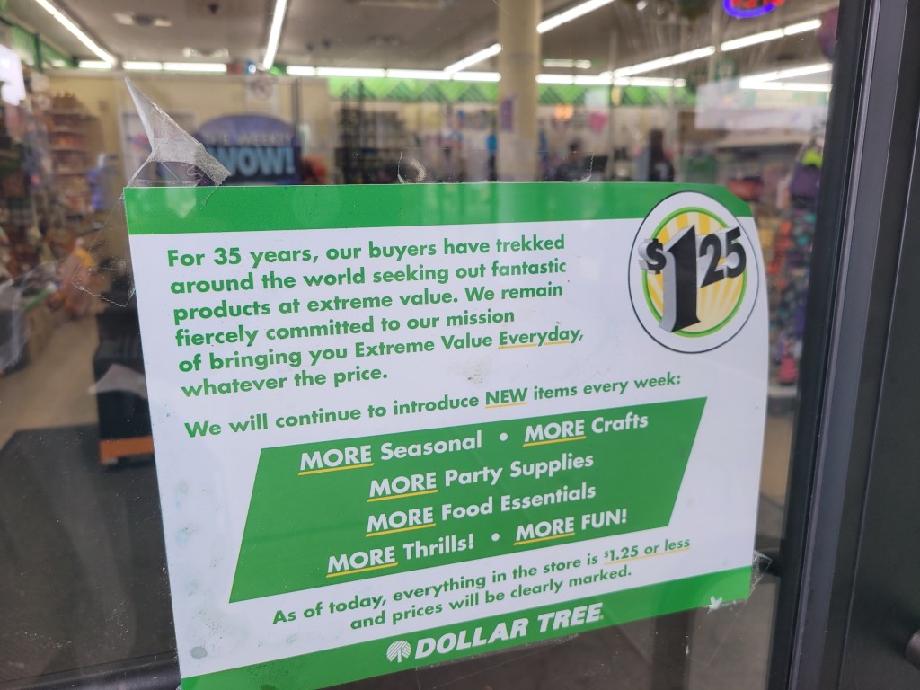
For years, all the products for sale in Dollar Tree stores had a price of $1.00 or less. But as inflation increased, the company had to raise its maxium prices to $1.25. (Thanks to Lena Buonanno for sending us the photo.)
There are multiple ways to measure inflation. Economists and policymakers use different measures of inflation depending on the use they intend to put the measure of inflation to. For example, as we discuss in Macroeconomics, Chapter 9, Section 9.4 (Economics, Chapter 19, Section 19.4), the Bureau of Labor Statistics (BLS) constructs the consumer price index (CPI) as measure of the cost of living of a typical urban household. So the BLS intends the percentage change in the CPI to measure inflation in the cost of living as experienced by the roughly 93 percent of the population that lives in an urban household. (We are referring here to what the BLS labels CPI–U. As we discuss in this blog post, the BLS also compiles a CPI for urban wage earners and clerical workers (or CPI–W).)
As we discuss in an Apply the Concept in Chapter 15, Section 15.5, because the Fed is charged by Congress with ensuring stability in the general price level, the Fed is interested in a broader measure of inflation than the CPI. So its preferred measure of inflation is the personal consumption expenditures (PCE) price index, which the Bureau of Economic Analysis (BEA) issues monthly. The PCE price index is a measure of the price level similar to the GDP deflator, except it includes only the prices of goods and services from the consumption category of GDP. Because the PCE price index includes more goods and services than the CPI, it is suits the Fed’s need for a broader measure of inflation. The Fed uses changes in the PCE to evaluate whether it’s meeting its target of a 2 percent annual inflation rate.
In using either the percentage change in the CPI or the percentage change in the PCE, we are looking at what inflation has been over the previous year. But economists and policymakers are also looking for indications of what inflation may be in the future. Prices of food and energy are particularly volatile, so the BLS issues data on the CPI excluding food and energy prices and the BEA does the same with respect to the PCE. These two measures help avoid the problem that, for example, a period of high gasoline prices might lead the inflation rate to temporarily increase. Note that inflation caclulated by excluding the prices of food and energy is called core inflation.
During the surge in inflation that began in the spring of 2021 and continued into the fall of 2022, some economists noted that supply chain problems and other effects of the pandemic on labor and product markets caused the prices of some goods and services to spike. For example, a shortage of computer chips led to a reduction in the supply of new cars and sharp increases in car prices. As with temporary spikes in prices of energy and food, spikes resulting from supply chain problems and other effects of the pandemic might lead the CPI and PCE—even excluding food and energy prices—to give a misleading measure of the underlying rate of inflation in the economy.
To correct for this problem, some economists have been more attention to the measure of inflation calculated using the median CPI, which is compiled monthly by economists at the Federal Reserve Bank of Cleveland. The median CPI is calculated by ranking the price changes of every good or service in the index from the largest price change to the smallest price change, and then choosing the price change in the middle. The idea is to eliminate the effect on measured inflation of any short-lived events that cause the prices of some goods and services to be particularly high or particularly low. Economists at the Cleveland Fed have conducted research that shows that, in their words, “the median CPI provides a better signal of the underlying inflation trend than either the all-items CPI or the CPI excluding food and energy. The median CPI is even better at forecasting PCE inflation in the near and longer term than the core PCE price index.”
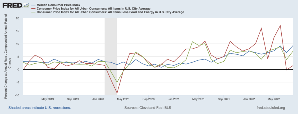
The following figure shows the three measures of inflation using the CPI for each month since January 2019. The red line shows the unadjusted CPI, the green line shows the CPI excluding food and energy prices, and the blue line shows median CPI. To focus on the inflation rate in a particular month, in this figure we calculate inflation as the percentage change in the index at an annual rate. That is, we calculate the annual inflation rate assuming that the inflation rate in that month continued for a year.
Note that for most of the period since early 2021, during which the inflation rate accelerated, median inflation was well below inflation measured by changes in the unadjusted CPI. That difference reflects some of the distortions in measuring inflation arising from the effects of the pandemic.
But the last two values—for July and August 2022—tell a different story. In those months, inflation measured by changes in the CPI excluding food and energy prices or by changes in median CPI were well above inflation measured by changes in the unadjusted CPI. In August 2022, the unadjusted CPI shows a low rate of inflation—1.4 percent—whereas the CPI excluding food and energy prices shows an inflation rate of 7.0 percent and the median CPI shows an inflation rate of 9.2 percent.
We should always be cautious when interpreting any economic data for a period as short as two months. But data for inflation measured by the change in median CPI may be sending a signal that the slowdown in inflation that many economists and policymakers had been predicting would occur in the summer of 2022 isn’t actually occurring. We’ll have to await the release of future data to draw a firmer conclusion.
Sources: Michael S. Derby, “Inflation Data Scrambles Fed Rate Outlook Again,” Wall Street Journal, September 14, 2022; Federal Reserve Bank of Cleveland, “Median CPI,” clevelandfed.org; and Federal Reserve Bank of St. Louis.
Supports: Macroeconomics, Chapter 9, Section 9.1,Economics Chapter 19, Section 19.1, and Essentials of Economics, Chapter 13, Section 13.1.
As it does on the first Friday of each month, on September 2, 2022, the U.S. Bureau of Labor Statistics (BLS) released its “Employment Situation” report for August 2022. According to the household survey data in the report, total employment in the U.S. economy increased in August by 442,000 compared with July. The unemployment rate rose from 3.5 percent in July to 3.7 percent in August. According to the establishment survey, the total number of workers on payrolls increased in August by 315,000 compared with July.
How are the data in the household survey collected? How are the data in the establishment survey collected?
Why are the estimated increases in employment from July to August 2022 in the two surveys different?
Briefly explain how it is possible for the household survey to report in a given month that both total employment and the unemployment rate increased.
Solving the Problem
Step 1: Review the chapter material. This problem is about how the BLS reports data on employment and unemployment, so you may want to review Chapter 9, Section 9.1, “Measuring the Unemployment Rate, the Labor Force Participation Rate, and the Employment–Population Ratio.”
Step 2: Answer part a. by explaining how the data from the two surveys are collected. As discussed in Section 9.1, the data in the household survey is from interviews with a sample of 60,000 households, chosen to represent the U.S. population. The data in the establishment survey—sometimes called the payroll survey in media stories—is from a sample of 300,000 establishments (factories, stores, and offices).
Step 3: Answer part b. by explaining why the estimated increase in employment is different in the two surveys. First note that the BLS intends the surveys to estimate two different measures of employment. The household survey includes people working at jobs of all types, including people who are self-employed or who are unpaid family workers, whereas the establishment survey includes only people who appear on a non-agricultural firm’s payroll, so the self-employed, farm workers, and unpaid family workers aren’t counted. Second, the data are collected from surveys and so—like all estimates that rely on surveys—will have some measurement error. That is, the actual increase in employment—either total employment in the household survey or payroll employment in the establishment survey—is likely to be larger or smaller than the reported estimates. The estimates in the establishment survey are revised in later months as the BLS receives additional data on payroll employment. In contrast, the estimates in household survey are ordinarily not revised because they are based only on a survey conducted once per month.
Step 4: Answer part c. by explaining how in a given month the household survey may report an increase in both employment and the unemployment rate. The BLS’s estimate of the unemployment is calculated from responses to the household survey. (The establishment survey doesn’t report an estimate of the unemployment rate.) The unemployment rate equals the total number of people unemployed divided by the labor force, multiplied by 100. The labor force equals the sum of the employed and the unemployed. If the number of people employed increases—thereby increasing the denominator in the unemployment rate equation—while the number of people unemployed remains the same or falls, as a matter of arithmetic the unemployment rate will have to fall.
The BLS reported that the unemployment rate in August 2022 rose even though total employment increased. That outcome is possible only if the number of people who are unemployed also increased, resulting in a proportionally larger increase in the numerator in the unemployment equation relative to the denominator. In fact, the BLS estimated that the number of people unemployed increased by 344,000 from July to August 2022. Employment and unemployment both increasing during a month happens fairly often during an economic expansion as some people who had been out of the labor force—and, therefore, not counted by the BLS as being unemployed—begin to search for work during the month but don’t find jobs.
Source: U.S. Bureau of Labor Statistics, “The Employment Situation—August 2022,” bls.gov, September 2, 2022.
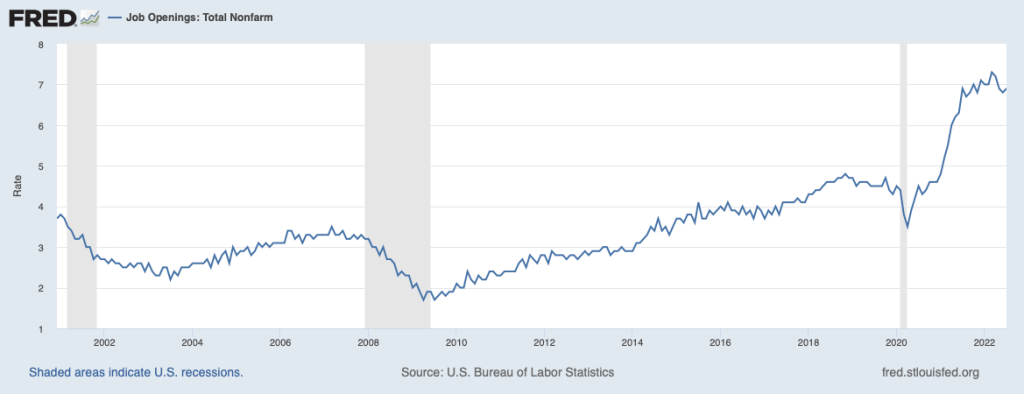
On Tuesday, August 30, 2022, the U.S. Bureau of Labor Statistics (BLS) released its Job Openings and Labor Turnover Survey (JOLTS) report for July 2022. The report indicated that the U.S. labor market remained very strong, even though, according to the Bureau of Economic Analysis (BEA), real gross domestic product (GDP) had declined during the first half of 2022. (In this blog post, we discuss the possibility that during this period the real GDP data may have been a misleading indicator of the actual state of the economy.)
As the following figure shows, the rate of job openings remained very high, even in comparison with the strong labor market of 2019 and early 2020 before the Covid-19 pandemic began disrupting the U.S. economy. The BLS defines a job opening as a full-time or part-time job that a firm is advertising and that will start within 30 days. The rate of job openings is the number of job openings divided by the number of job openings plus the number of employed workers, multiplied by 100.
In the following figure, we compare the total number of job openings to the total number of people unemployed. The figure shows that in July 2022 there were almost two jobs available for each person who was unemployed.
Typically, a strong job market with high rates of job openings indicates that firms are expanding and that they expect their profits to be increasing. As we discuss in Macroeconomics, Chapter 6, Section 6.2 (Microeconomics and Economics, Chapter 8, Section 8.2) the price of a stock is determined by investors’ expectations of the future profitability of the firm issuing the stock. So, we might have expected that on the day the BLS released the July JOLTS report containing good news about the labor market, the stock market indexes like the Dow Jones Industrial Average, the S&P 500, and the Nasdaq Composite Index would rise. In fact, though the indexes fell, with the Dow Jones Industrial Average declining a substantial 300 points. As a column in the Wall Street Journal put it: “A surprisingly tight U.S. labor market is rotten news for stock investors.” Why did good news about the labor market could cause stock prices to decline? The answer is found in investors’ expectations of the effect the news would have on monetary policy.
In August 2022, Fed Chair Jerome Powell and the other members of the Federal Reserve Open Market Committee (FOMC) were in the process of tightening monetary policy to reduce the very high inflation rates the U.S. economy was experiencing. In July 2022, inflation as measured by the percentage change in the consumer price index (CPI) was 8.5 percent. Inflation as measured by the percentage change in the personal consumption expenditures (PCE) price index—which is the measure of inflation that the Fed uses when evaluating whether it is hitting its target of 2 percent annual inflation—was 6.3 percent. (For a discussion of the Fed’s choice of inflation measure, see the Apply the Concept “Should the Fed Worry about the Prices of Food and Gasoline,” in Macroeconomics, chapter 15, Section 15.5 and in Economics, Chapter 25, Section 25.5.)
To slow inflation, the FOMC was increasing its target for the federal funds rate—the interest rate that banks charge each other on overnight loans—which in turn was leading to increases in other interest rates, such as the interest rate on residential mortgage loans. Higher interest rates would slow increases in aggregate demand, thereby slowing price increases. How high would the FOMC increase its target for the federal funds rate? Fed Chair Powell had made clear that the FOMC would monitor economic data for indications that economic activity was slowing. Members of the FOMC were concerned that unless the inflation rate was brought down quickly, the U.S. economy might enter a wage-price spiral in which high inflation rates would lead workers to push for higher wages, which, in turn, would increase firms’ labor costs, leading them to raise prices further, in response to which workers would push for even higher wages, and so on. (We discuss the concept of a wage-price spiral in this earlier blog post.)
In this context, investors interpretated data showing unexpected strength in the economy—particularly in the labor market—as making it likely that the FOMC would need to make larger increases in its target for the federal fund rate. The higher interest rates go, the more likely that the U.S. economy will enter an economic recession. During recessions, as production, income, and employment decline, firms typically experience lower profits or even suffer losses. So, a good JOLTS report could send stock prices falling because news that the labor market was stronger than expected increased the likelihood that the FOMC’s actions would push the economy into a recession, reducing profits. Or as the Wall Street Journal column quoted earlier put it:
“So Tuesday’s [JOLTS] report was good news for workers, but not such good news for stock investors. It made another 0.75-percentage-point rate increase [in the target for the federal funds rate] from the Fed when policy makers meet next month seem increasingly likely, while also strengthening the case that the Fed will keep raising rates well into next year. Stocks sold off sharply following the report’s release.”
Sources: U.S. Bureau of Labor Statistics, “Job Openings and Labor Turnover–July 2022,” bls.gov, August 30, 2022; Justin Lahart, “Why Stocks Got Jolted,” Wall Street Journal, August 30, 2022; Jerome H. Powell, “Monetary Policy and Price Stability,” speech at “Reassessing Constraints on the Economy and Policy,” an economic policy symposium sponsored by the Federal Reserve Bank of Kansas City, Jackson Hole, Wyoming, August 26, 2022; and Federal Reserve Bank of St. Louis.
The Bureau of Economic Analysis (BEA) publishes data on gross domestic product (GDP) each quarter. Economists and media reports typically focus on changes in real GDP as the best measure of the overall state of the U.S. economy. But, as we discuss in Macroeconomics, Chapter 8, Section 8.4 (Economics, Chapter 18, Section 18.4), the BEA also publishes quarterly data on gross domestic income (GDI). As we discuss in Chapter 8, Section 8.1 when discussing the circular-flow diagram, the value of every final good and services produced in the economy (GDP) should equal the value of all the income in the economy resulting from that production (GDI). The BEA has designed the two measures to be identical by including in GDI some non-income items, such as sales taxes and depreciation. But as we discuss in the Apply the Concept, “Should We Pay More Attention to Gross Domestic Income?” GDP and GDI are compiled by the BEA from different data sources and can sometimes significantly diverge.
A large divergence between the two measures occurred in the first half of 2022. During this period real GDP declined—as shown by the blue line in the following figure—after which some stories in the media indicated that the U.S. economy was in a recession. But real GDI—as shown by the red line in the figure—increased during the same two quarters. So, was the U.S. economy still in the expansion that began in the third quarter of 2020, rather than in a recession? Or, as an article in the Wall Street Journal put it: “A Different Take on the U.S. Economy: Maybe It Isn’t Really Shrinking.”
In fact, most economists do not follow the popular definition of a recession as being two consecutive quarters of declining real GDP. Instead, as we discuss in Chapter 10, Section 10.3, economists typically follow the definition of a recession used by the National Bureau of Economic Research: “A recession is a significant decline in activity spread across the economy, lasting more than a few months, visible in industrial production, employment, real income, and wholesale-retail trade.”
During the first half of 2022, most measures of economic activity were expanding, rather than contracting. For example, the first of the following figures shows payroll employment increasing in each month in the first half of 2022. The second figure shows industrial production also increasing during most months in the first half of 2022, apart from a very slight decline from April to May after which it continued to increase.
Taken together, these data indicate that the U.S. economy was likely not in a recession during the first half of 2022. The BEA revises the data on real GDP and real GDI over time as various government agencies gather more information on the different production and income measures included in the series. Jeremy Nalewaik of the Federal Reserve Board of Governors has analyzed the BEA’s adjustments to its initial estimates of real GDP and real GDI. He has found that when there are significant differences between the two series, the BEA revisions usually result in the GDP values being revised to be closer to the GDI values. Put another way, the initial GDI estimates may be more accurate than the initial GDP estimates.
If that generalization holds true in 2022, then the BEA may eventually revise its estimates of GDP upward, which would show that the U.S. economy was not in a recession in the first of half of 2022 because economic activity was increasing rather than decreasing.
Sources: Jon Hilsenrath, “A Different Take on the U.S. Economy: Maybe It Isn’t Really Shrinking,” Wall Street Journal, August 28, 2022; Reade Pickert, “Key US Growth Measures Diverge, Complicating Recession Debate,” bloomberg.com, August 25, 2022; Jeremy L. Nalewaik, “The Income- and Expenditure-Side Estimates of U.S. Output Growth,” Brookings Papers on Economic Activity, Spring 2010, pp. 71-127; and Federal Reserve Bank of St. Louis.
In the textbook, we discuss several measures of inflation. In Macroeconomics, Chapter 8, Section 8.4 (Economics, Chapter 18, Section 18.4) we discuss the GDP deflator as a measure of the price level and the percentage change in the GDP deflator as a measure of inflation. In Chapter 9, Section 9.4, we discuss the consumer price index (CPI) as a measure of the price level and the percentage change in the CPI as the most widely used measure of inflation.
In Chapter 15, Section 15.5 we examine the reasons that the Federal Reserve often looks at the core inflation rate—the inflation rate excluding the prices of food and energy—as a better measure of the underlying rate of inflation. Finally, in that section we note that the Fed uses the percentage change in the personal consumption expenditures (PCE) price index to assess of whether it’s achieving its goal of a 2 percent inflation rate.
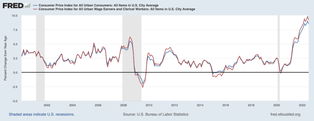
In this blog post, we’ll discuss two other aspects of measuring inflation that we don’t cover in the textbook. First, the Bureau of Labor Statistics (BLS) publishes two versions of the CPI: (1) The familiar CPI for all urban consumers (or CPI–U), which includes prices of goods and services purchased by households in urban areas, and (2) the less familiar CPI for urban wage earners and clerical workers (or CPI–W), which includes the same prices included in the CPI–U. The two versions of the CPI give slightly different measures of the inflation rate—despite including the same prices—because each version applies different weights to the prices when constructing the index.
As we explain in Chapter 9, Section 9.4, the weights in the CPI–U (the only version of the CPI we discuss in the chapter) are determined by a survey of 36,000 households nationwide on their spending habits. The more the households surveyed spend on a good or service, the larger the weight the price of the good or service receives in the CPI–U. To calculate the weights in the CPI–W the BLS uses only expenditures by households in which at least half of the household’s income comes from a clerical or wage occupation and in which at least one member of the household has worked 37 or more weeks during the previous year. The BLS estimates that the sample of households used in calculating the CPI–U includes about 93 percent of the population of the United States, while the households included in the CPI–W include only about 29 percent of the population.
Because the percentage of the population covered by the CPI–U is so much larger than the percentage of the population covered by the CPI–W, it’s not surprising that most media coverage of inflation focuses on the CPI–U. As the following figure shows, the measures of inflation from the two versions of the CPI aren’t greatly different, although inflation as measured by the CPI–W—the red line—tends to be higher during economic expansions and lower during economic recessions than inflation measured by the CPI–U—the blue line.
One important use of the CPI–W is in calculating cost-of-living adjustments (COLAs) applied to Social Security payments retired and disabled people receive. Each year, the federal government’s Social Security Administration (SSA) calculates the average for the CPI–W during June, July, and August in the current year and in the previous year and then measures the inflation rate as the percentage increase between the two averages. The SSA then increases Social Security payments by that inflation rate. Because the increase in CPI–W is often—although not always—larger than the increase in CPI–U, using CPI–W to calculate Social Security COLAs increases the payments recipients of Social Security receive.
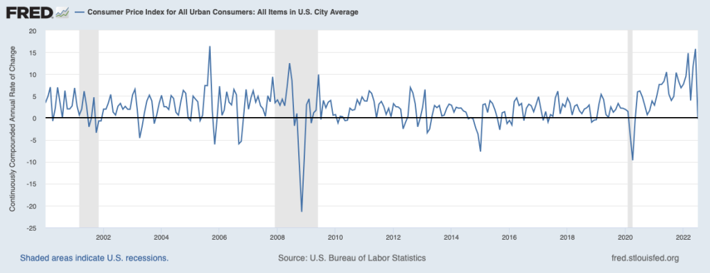
A second aspect of measuring inflation that we don’t mention in the textbook was the subject of discussion following the release of the July 2022 CPI data. In June 2022, the value for the CPI–U was 295.3. In July 2022, the value for the CPI–U was also 295.3. So, was there no inflation during July—an inflation rate of 0 percent? You can certainly make that argument, but typically, as we note in the textbook (for instance, see our display of the inflation rate in Chapter 10, Figure 10.7) we measure the inflation rate in a particular month as the percentage change in the CPI from the same month in the previous year. Using that approach to measuring inflation, the inflation rate in July 2022 was the percentage change in the CPI from its value in July 2021, or 8.5 percent. Note that you could calculate an annual inflation rate using the increase in the CPI from one month to the next by compounding that rate over 12 months. In this case, because the CPI was unchanged from June to July 2022, the inflation rate calculated as a compound annual rate would be 0 percent.
During periods of moderate inflation rates—which includes most of the decades prior to 2021—the difference between inflation calculated in these two ways was typically much smaller. Focusing on just the change in the CPI for one month has the advantage that you are using only the most recent data. But if the CPI in that month turns out to be untypical of what is happening to inflation over a longer period, then focusing on that month can be misleading. Note also that inflation rate calculated as the compound annual change in the CPI each month results in very large fluctuations in the inflation rate, as shown in the following figure.
Sources: Anne Tergesen, “Social Security Benefits Are Heading for the Biggest Increase in 40 Years,” Wall Street Journal, August 10, 2022; Neil Irwin, “Inflation Drops to Zero in July Due to Falling Gas Prices,” axios.com, August 10, 2022; “Consumer Price Index Frequently Asked Questions,” bls.gov, March 23, 2022; Stephen B. Reed and Kenneth J. Stewart, “Why Does BLS Provide Both the CPI–W and CPI–U?” U.S. Bureau of Labor Statistics, Beyond the Numbers, Vol. 3, No. 5, February 2014; “Latest Cost of Living Adjustment,” ssa.gov; and Federal Reserve Bank of St. Louis.
Senator Elizabeth Warren (Photo from the Associated Press)Lawrence Summers (Photo from harvardmagazine.com)
As we’ve discussed in several previous blog posts, in early 2021 Lawrence Summers, professor of economics at Harvard and secretary of the treasury in the Clinton administration, argued that the Biden administration’s $1.9 trillion American Rescue Plan, enacted in March, was likely to cause a sharp acceleration in inflation. When inflation began to rapidly increase, Summers urged the Federal Reserve to raise its target for the federal funds rate in order to slow the increase in aggregate demand, but the Fed was slow to do so. Some members of the Federal Open Market Committee (FOMC) argued that much of the inflation during 2021 was transitory in that it had been caused by lingering supply chain problems initially caused by the Covid–19 pandemic.
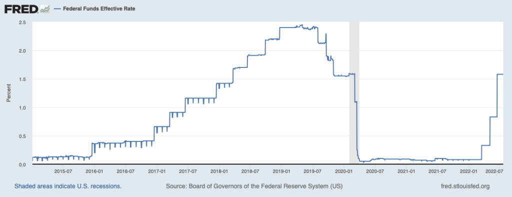
At the beginning of 2022, most members of the FOMC became convinced that in fact increases in aggregate demand were playing an important role in causing high inflation rates. Accordingly, the FOMC began increasing its target for the federal funds rate in March 2022. After two more rate increases, on the eve of the FOMC’s meeting on July 26–27, the federal funds rate target was a range of 1.50 percent to 1.75 percent. The FOMC was expected to raise its target by at least 0.75 percent at the meeting. The following figure shows movements in the effective federal funds rate—which can differ somewhat from the target rate—from January 1, 2015 to July 21, 2022.
In an opinion column in the Wall Street Journal, Massachusetts Senator Elizabeth Warren argued that the FOMC was making a mistake by increasing its target for the federal funds rate. She also criticized Summers for supporting the increases. Warren worried that the rate increases were likely to cause a recession and argued that Congress and President Biden should adopt alternative measures to contain inflation. Warren argued that a better approach to dealing with inflation would be to, among other steps, increase the federal government’s support for child care to enable more parents to work, provide support for strengthening supply chains, and lower prescription drug prices by allowing Medicare to negotiate the prices with pharmaceutical firms. She also urged a “crack down on price gouging by large corporations.” (We discussed the argument that monopoly power is responsible for inflation in this blog post.)
Summers responded to Warren in a Twitter thread. He noted that: “In the 18 months since the massive stimulus policies & easy money that [Senator Warren] has favored & I have opposed, the inflation rate has risen from below 2 to above 9 percent & workers purchasing power has, as a consequence, declined more rapidly than in any year in the last 50.” And “[Senator Warren] opposes restrictive monetary policy or any other measure to cool off total demand. Why does she think at a time when there are twice as many vacancies as jobs that inflation will come down without some drop in total demand?”
Clearly, economists and policymakers continue to hotly debate monetary policy.
Source: Elizabeth Warren, “Jerome Powell’s Fed Pursues a Painful and Ineffective Inflation Cure,” Wall Street Journal, July 24, 2022.