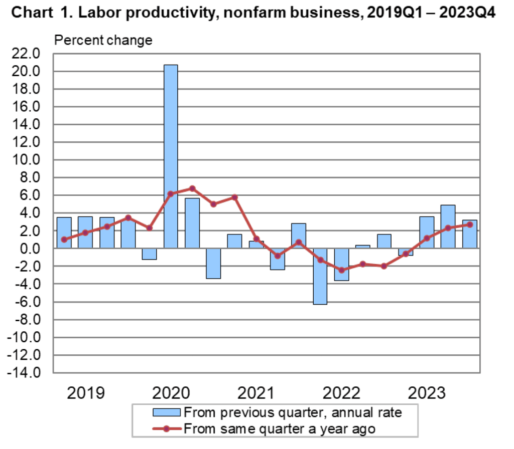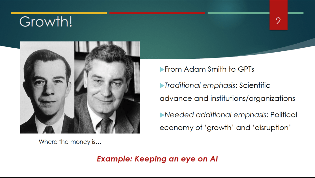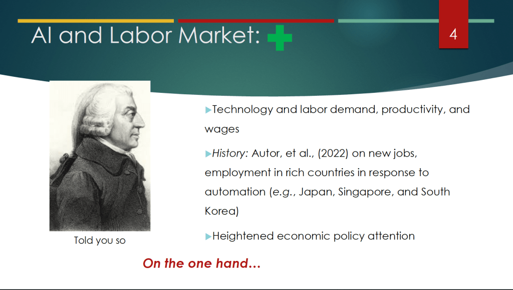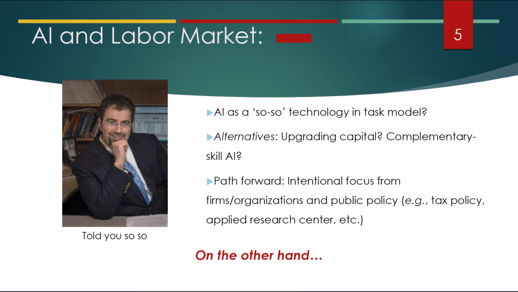
Glenn’s Presentation at the ASSA Session on “The U.S. Economy: Growth, Stagnation or Financial Crisis and Recession?”

Glenn participated in this session hosted by the Society of Policy Modeling and the American Economic Association of Economic Educators and moderated by Dominick Salvatore of Fordham University. (Link to the page for this session in the ASSA program.)

Also making presentations at the session were Robert Barro of Harvard University, Janice Eberly of Northwestern University, Kenneth Rogoff of Harvard University, and John Taylor of Stanford University.

Here is the abstract for Glenn’s presentation:

Economic growth is foundational for living standards and as an objective for economic policy. The emergence of Artificial Intelligence as a General Purpose Technology, on the one hand, and a number of demographic and budget challenges, on the other hand, generate an unusually wide range of future economic outcomes. I focus on key ‘policy’ and ‘political economy’ considerations that increase the likelihood of a more favorable growth path given pre-existing trends and technological possibilities. By ‘policy,’ I consider mechanisms enabling growth through research, taxation, the scope of regulation, and competition. By ‘political economy’ factors, I consider mechanisms to increase economic participation in support of growth and policies that enhance it. I argue that both sets of mechanisms are necessary for a viable pro-growth economic policy framework.

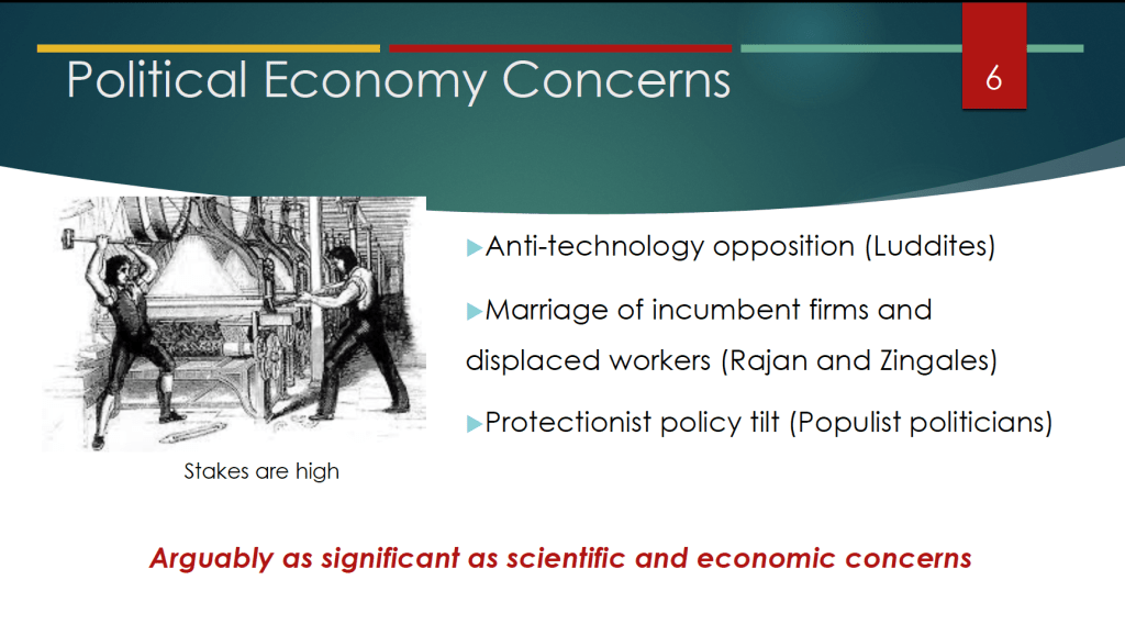
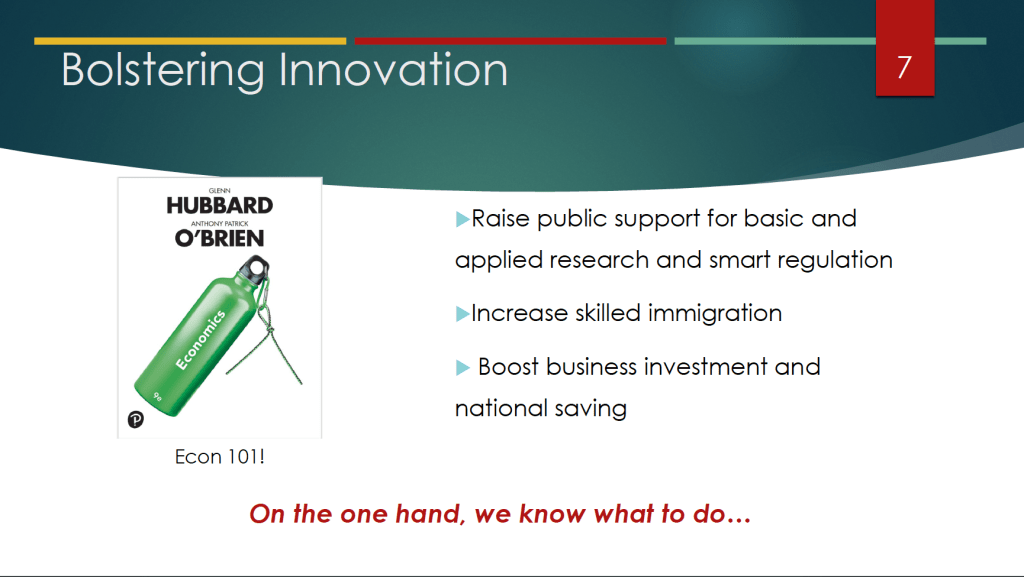
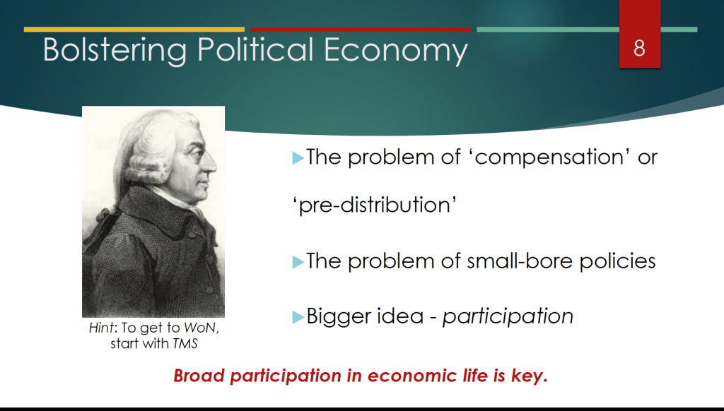
These slides from the presentation highlight some of Glenn’s key points. (Note the cover of the new 9th edition of the textbook in slide 7!)

Glenn, Harry Holzer, and Michael Strain Analyze the Effect of Changes in Unemployment Benefits during the Pandemic

A job fair in Jackson, Mississippi (photo from the Associated Press)

As part of the Social Security Act of 1935,Congress created the unemployment insurance program to make payments to unemployed workers. The program run jointly by the federal government and the state governments. It’s financed primarily by state and federal taxes on employers. States are allowed to determine which workers are eligible, the dollar amount of the unemployment benefit workers will receive, and for how long workers will receive the benefit. 

 What’s the purpose of the unemployment insurance program? A document published the U.S. Department of Labor explains that: “Unemployment compensation is a social insurance program. It is designed to provide benefits to most individuals out of work, generally through no fault of their own, for periods between jobs…. [Unemployment compensation] ensures that a significant proportion of the necessities of life can be met on a week-to-week basis while a search for work takes place.”

But the same document also notes that unemployment compensation “maintains [unemployed workers’] purchasing power which also acts as an economic stabilizer in times of economic downturn.” By “economic stabilizer,” the Department of Labor is noting that unemployment compensation is what in Macroeconomics, Chapter 16, Section 16.1 (Economics, Chapter 26, Section 26.1) we call an automatic stabilizer. An automatic stabilizer is a government spending or taxing program that automatically increases or decreases along with the business cycle.  

As shown in the following figure, when the economy enters a recession, the total amount of unemployment compensation payments increases without the federal government or the state governments having to take any action because eligibility for the payments is already defined in existing law. So, during a recession, the unemployment insurance program helps to keep aggregate demand higher than it would otherwise be, which can lessen the severity of the recession.  

As we discuss in Macroeconomics, Chapter 9, Section 9.3 (Economics, Chapter 19, Section 19.3), the unemployment insurance program can have an unintended effect. The higher the unemployment insurance payment a worker receives and the longer the worker receives it, the more likely the worker is to delay searching for another job. In other words, by reducing the opportunity cost of being unemployed, unemployment insurance benefits may unintentionally increase the length of unemployment spells—the amount of time the typical worker is unemployed. 

During and immediately after the 2020 recession, the federal government increased the dollar amount of the unemployment insurance payments that workers received and extended the number of months workers could continue to receive these payments.  Under the American Rescue Plan, a law which President Biden proposed and Congress passed in March 2021, workers receiving unemployment insurance benefits received an additional $300 weekly from March 2021 until September 6, 2021. Also, under the law, people, such as the self-employed and gig workers, would receive unemployment insurance benefits even though they had previously been ineligible to receive them. (Note the resulting spike during this period in the total dollar amount of unemployment insurance benefits as shown in the above figure.)

Some state governments were concerned that the extended benefits might cause some workers to delay taking jobs, thereby slowing the recovery of these states’ economies from the effects of the pandemic. Accordingly, 18 states stopped participating in the programs in June 2021, meaning that at that time unemployed workers would no longer receive the extra $300 per week and workers who prior to March 2021 hadn’t been eligible to receive unemployment benefits would again be ineligible.

Were unemployed workers in the states that ended the expanded unemployment insurance benefits in June more likely to become employed than were unemployed workers in states that continued the expanded benefits into September? On the one hand, ending the expanded benefits would increase the opportunity cost of not having a job. But, on the other hand, because government payments to workers would decline in these states, the result could be a decline in consumer spending that would decrease the demand for labor.  Which of these effects was larger would determine whether employment increased or decreased in the states that ended expanded unemployment benefits early.

Glenn, along with Harry Holzer of Georgetown University and Michael Strain of the American Enterprise Institute, carried out an econometric analysis to explore the effects ending expanded unemployment benefits early had on the labor markets in those states.  They find that:

  1. Among unemployed workers ages 25 to 54 (“prime-age workers”), ending the expanded unemployment benefit program increased the number of workers in those states who moved from being unemployed to being employed by 14 percentage points.
  2. Among prime-age workers, the employment-to-population ratio in those states increased by about 1 percentage point.
  3. Among prime-age workers, the unemployment rate in those stated decreased by about 0.9 percentage point.

These estimates indicate that the effect of ending the expanded unemployment benefit program raised the opportunity cost of being unemployed more than it decreased the demand for labor by reducing the incomes of some household. But what about the larger question of whether households were made better or worse off as a result of ending the program early? The authors find that ending the program early decreased the share of households that had no difficulty meeting expenses. They, therefore, conclude that the effects on household well-being of ending the program early are ambiguous. 

The paper presenting these results can be found here. Warning! The econometric analysis is quite technical.

The Roman Emperor Vespasian Fell Prey to the Lump-of-Labor Fallacy

Bust of the Roman Emperor Vespasian. (Photo from en.wikipedia.org.)

Some people worry that advances in artificial intelligence (AI), particularly the development of chatbots will permanently reduce the number of jobs available in the United States. Technological change is often disruptive, eliminating jobs and sometimes whole industries, but it also creates new industries and new jobs. For example, the development of mass-produced, low-priced automobiles in the early 1900s wiped out many jobs dependent on horse-drawn transportation, including wagon building and blacksmithing. But automobiles created many new jobs not only on automobile assembly lines, but in related industries, including repair shops and gas stations.

Over the long run, total employment in the United States has increased steadily with population growth, indicating that technological change doesn’t decrease the total amount of jobs available. As we discuss in Microeconomics, Chapter 16 (also Economics, Chapter 16), fears that firms will permanently reduce their demand for labor as they increase their use of the capital that embodies technological breakthroughs, date back at least to the late 1700s in England, when textile workers known as Luddites—after their leader Ned Ludd—smashed machinery in an attempt to save their jobs. Since that time, the term Luddite has described people who oppose firms increasing their use of machinery and other capital because they fear the increases will result in permanent job losses.

Economists believe that these fears often stem from the lump-of-labor fallacy, which holds that there is only a fixed amount of work to be performed in the economy. So the more work that machines perform, the less work that will be available for people to perform. As we’ve noted, though, machines are substitutes for labor in some uses—such as when chatbot software replace employees who currently write technical manuals or computer code—they are also complements to labor in other jobs—such as advising firms on how best to use chatbots. 

The lump-of-labor fallacy has a long history, probably because it seems like common sense to many people who see the existing jobs that a new technology destroys, without always being aware of the new jobs that the technology creates. There are historical examples of the lump-of-labor fallacy that predate even the original Luddites.

For instance, in his new book Pax: War and Peace in Rome’s Golden Age, the British historian Tom Holland (not to be confused with the actor of the same name, best known for portraying Spider-Man!), discusses an account by the ancient historian Suetonius of an event during the reign of Vespasian who was Roman emperor from 79 A.D. to 89 A.D. (p. 201):

“An engineer, so it was claimed, had invented a device that would enable columns to be transported to the summit of the [Roman] Capitol at minimal cost; but Vespasian, although intrigued by the invention, refused to employ it. His explanation was a telling one. ‘I have a duty to keep the masses fed.’”

Vespasian had fallen prey to the lump-of-labor fallacy by assuming that eliminating some of the jobs hauling construction materials would reduce the total number of jobs available in Rome. As a result, it would be harder for Roman workers to earn the income required to feed themselves.

Note that, as we discuss in Macroeconomics, Chapters 10 and 11 (also Economics, Chapter 20 and 21), over the long-run, in any economy technological change is the main source of rising incomes. Technological change increases the productivity of workers and the only way for the average worker to consume more output is for the average worker to produce more output. In other words, most economists agree that the main reason that the wages—and, therefore, the standard of living—of the average worker today are much higher than they were in the past is that workers today are much more productive because they have more and better capital to work with.

Although the Roman Empire controlled most of Southern and Western Europe, the Near East, and North Africa for more than 400 years, the living standard of the average citizen of the Empire was no higher at the end of the Empire than it had been at the beginning. Efforts by emperors such as Vespasian to stifle technological progress may be part of the reason why. 

Claudia Goldin Wins the Nobel Prize in Economics

Claudia Goldin (Photo from Goldin’s web page at havard.edu.)

Claudia Goldin, the Henry Lee Professor of Economics at Harvard, has been awarded the 2023 Nobel Prize in Economic Sciences. Goldin’s research is wide-ranging, with a focus on the economic history of women and on gender disparities in wages and employment. She received her PhD from the University of Chicago in 1972 for a thesis that was published in 1976 as Urban Slavery in the American South, 1820 to 1860: A Quantitative History. Her thesis adviser, Robert Fogel, was awarded the Nobel Prize in 1993 for his work in economic history. He shared the prize that year with Douglas North of Washington University in St. Louis. Goldin’s work on economic history contributed to the cliometric revolution, which involves the application of theoretical models and econometric methods to the study of historical issues.  At the time of the award to Fogel and North, Goldin discussed their research and the cliometric revolution here.

Goldin’s pioneering and influential research on the economic history of women was the basis for her 1990 book Understanding the Gender Gap: An Economic History of American Women. The themes of that book were expanded on in 2021 in Career & Family: Women’s Century-Long Journey toward Equity, and in her forthcoming An Evolving Force: A History of Women in the Economy.

In research with Lawrence Katz, also a professor of economics at Harvard, Goldin has explored how technological change and educational attainment have affected income inequality, particularly the wage premium skilled workers receive. Goldin and Katz summarized their findings in 2008 in the influential book, The Race between Education and Technology.

The wide scope of Goldin’s research can be seen by reviewing her curriculum vitae, which can be found here. The announcement by the Nobel committee can be found here.

Data Indicate Continued Labor Market Easing

A job fair in Albuquerque, New Mexico earlier this year. (Photo from Zuma Press via the Wall Street Journal.)

In his speech at the Kansas City Fed’s Jackson Hole, Wyoming symposium, Fed Chair Jerome Powell noted that: “Getting inflation back down to 2 percent is expected to require a period of below-trend economic growth as well as some softening in labor market conditions.” To this point, there isn’t much indication that the U.S. economy is experiencing slower economic growth. The Atlanta Fed’s widely followed GDPNow forecast has real GDP increasing at a rapid 5.3 percent during the third quarter of 2023.

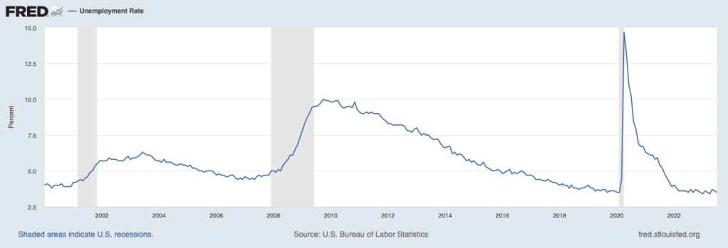
But the labor market does appear to be softening. The most familiar measure of the state of the labor market is the unemployment rate. As the following figure shows, the unemployment rate remains very low.

But, as we noted in this earlier post, an alternative way of gauging the strength of the labor market is to look at the ratio of the number of job openings to the number of unemployed workers. The Bureau of Labor Statistics (BLS) defines a job opening as a full-time or part-time job that a firm is advertising and that will start within 30 days. The higher the ratio of job openings to unemployed workers, the more difficulty firms have in filling jobs, and the tighter the labor market is. As indicated by the earlier quote from Powell, the Fed is concerned that in a very tight labor market, wages will increase more rapidly, which will likely lead firms to increase prices. The following figure shows that in July the ratio of job openings to unemployed workers has declined from the very high level of around 2.0 that was reached in several months between March 2022 and December 2022. The July 2023 value of 1.5, though, was still well above the level of 1.2 that prevailed from mid-2018 to February 2022, just before the beginning of the Covid–19 pandemic. These data indicate that labor market conditions continue to ease, although they remain tighter than they were just before the pandemic.

The following figure shows movements in the quit rate. The BLS calculates job quit rates by dividing the number of people quitting jobs by total employment. When the labor market is tight and competition among firms for workers is high, workers are more likely to quit to take another job that may be offering higher wages. The quit rate in July 2023 had fallen to 2.3 percent of total employment from a high of 3.0 percent, reached in both November 2021 and April 2022. The quit rate was back to its value just before the pandemic. The quit rate data are consistent with easing conditions in the labor market. (The data on job openings and quits are from the BLS report Job Openings and Labor Turnover—July 2023—the JOLTS report—released on August 29. The report can be found here.)

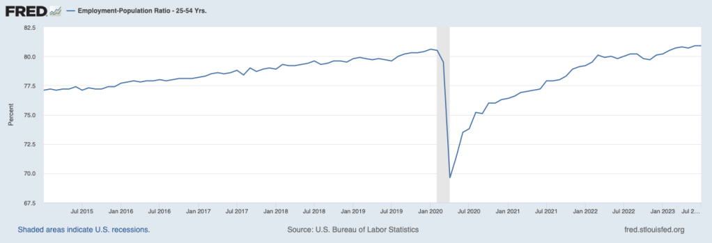
In his Jackson Hole speech, Powell noted that: “Labor supply has improved, driven by stronger participation among workers aged 25 to 54 and by an increase in immigration back toward pre-pandemic levels.” The following figure shows the employment-population ratio for people aged 25 to to 54—so-called prime-age workers. In July 2023, 80.9 percent of people in this age group were employed, actually above the ratio of 80.5 percent just before the pandemic. This increase in labor supply is another indication that the labor market disruptions caused by the pandemic has continued to ease, allowing for an increase in labor supply.

Taken together, these data indicate that labor market conditions are easing, likely reducing upward pressure on wages, and aiding the continuing decline in the inflation rate towards the Fed’s 2 percent target. Unless the data for August show an acceleration in inflation or a tightening of labor market conditions—which is certainly possible given what appears to be a strong expansion of real GDP during the third quarter—at its September meeting the Federal Open Market Committee is likely to keep its target for the federal funds rate unchanged.

The Effect on a Firm’s Costs of Using a Generative AI Program

Supports: Microeconomics, Chapter 11, Section 11.5; Economics, Chapter 11, Section 11.5; and Essentials of Economics, Chapter 8, Section 8.5

Photo from the Wall Street Journal.

Imani owns a firm that sells payroll services to companies in the Atlanta area. Her largest cost is for labor. She employs workers who use software to prepare payroll reports and to handle texts and calls from client firms. She decides to begin using a generative AI program, like ChatGPT, which is capable of quickly composing thorough answers to many questions and write computer code. She will use the program to write the additional computer code needed to adapt the payroll software to individual client’s needs and to respond to clients seeking advice on payroll questions. Once the AI program is in place, she will need only half as many workers. The number of additional workers she needs to hire for every 20 additional firms that buy her service will fall from 5 to 1. She will have to pay a flat monthly licensing fee for the AI program; the fee will not change with the number of firms she sells her services to. Imani determines that making these changes will reduce her total cost of providing services to her current 2,000 clients from $2,000,000 per month to $1,600,000 per month

In answering the following questions, assume that, apart from the number of workers, none of the other inputs—such as the size of her firm’s office, the number of computers, or other software—change as a result of her leasing the AI program.

a. Briefly explain whether each of the following statements about the cost situation at Imani’s firm after she begins using the AI program is correct or incorrect.

  1. Her firm’s average total cost, average variable cost, and average fixed cost curves will shift down, while her firm’s marginal cost curve will shift up.
  2. Her firm’s average total cost, average variable cost, average fixed cost and marginal cost curves will all shift up.
  3. Her firm’s average total cost, average variable cost, and marginal cost curves will shift down, while her average fixed cost curve will shift up.
  4. Her firm’s average total cost, average variable cost, average fixed cost, and marginal cost curves will all shift down.
  5. Her firm’s average fixed cost curve will shift up, but her other cost curves will be unchanged.

b. Draw a graph illustrating your answer to part a. Be sure to show the original average total cost, average variable cost, average fixed cost, and marginal cost curves. Also show the shifts—if any—in the curves after Imani begins using the AI program.

Solving the Problem

Step 1:  Review the chapter material. This problem requires you to understand definitions of costs, so you may want to review the sections “The Difference between Fixed Costs and Variable Costs,” “Marginal Costs,” and “Graphing Cost Curves”

Step 2:  Answer part (a) by explaining whether each of the five listed statements is correct or incorrect. The cost of the AI program is fixed because it doesn’t change with the quantity of her services that Imani sells. Her firm will have greater fixed costs after licensing the AI program but she will have lower variable costs because she is able to produce the same level of output with fewer workers. Her marginal cost will also decline because she needs to hire fewer workers as the quantity of services she sells increases. We know that the average total cost per month of providing her service to 2,000 clients has decreased because we are given the information that it changed from ($2,000,000/2,000) = $1,000 to ($1,600,000/2,000) = $800.

  1. This statement is incorrect because her average fixed cost curve will shift up as a result of her total fixed cost having increased by the amount of the AI program license and because her marginal cost curve will shift down, not up.
  2. This statement is incorrect because all of her cost curves, except for average fixed cost, will shift down, not up.
  3. This statement is correct because it describes the actual shifts in her cost curves. 
  4. This statement is incorrect because her average fixed cost curve will shift up, not down.
  5. This statement is incorrect because her rather than being unaffected, her average total cost, average variable cost, and marginal cost curves will shift down.

Step 3:  Answer part (b) by drawing the cost curves for Imani’s firm before and after she begins using the AI program. Your graph should look like the following, where the curves representing the firm’s costs before Imani begins leasing the AI program are in blue and the costs after leasing the program are in red. 

Solved Problem: How Can Total Employment and the Unemployment Rate Both Increase?

Photo from the New York Times.

Supports: Macroeconomics, Chapter 9, Section 9.1, Economics Chapter 19, Section 19.1, and Essentials of Economics, Chapter 13, Section 13.1.

As it does on the first Friday of each month, on September 2, 2022, the U.S. Bureau of Labor Statistics (BLS) released its “Employment Situation” report for August 2022. According to the household survey data in the report, total employment in the U.S. economy increased in August by 442,000 compared with July. The unemployment rate rose from 3.5 percent in July to 3.7 percent in August. According to the establishment survey, the total number of workers on payrolls increased in August by 315,000 compared with July.

  1. How are the data in the household survey collected? How are the data in the establishment survey collected?
  2. Why are the estimated increases in employment from July to August 2022 in the two surveys different? 
  3. Briefly explain how it is possible for the household survey to report in a given month that both total employment and the unemployment rate increased.

Solving the Problem

Step 1: Review the chapter material. This problem is about how the BLS reports data on employment and unemployment, so you may want to review Chapter 9, Section 9.1, “Measuring the Unemployment Rate, the Labor Force Participation Rate, and the Employment–Population Ratio.” 

Step 2: Answer part a. by explaining how the data from the two surveys are collected. As discussed in Section 9.1, the data in the household survey is from interviews with a sample of 60,000 households, chosen to represent the U.S. population. The data in the establishment survey—sometimes called the payroll survey in media stories—is from a sample of 300,000 establishments (factories, stores, and offices).  

Step 3: Answer part b. by explaining why the estimated increase in employment is different in the two surveys.  First note that the BLS intends the surveys to estimate two different measures of employment. The household survey includes people working at jobs of all types, including people who are self-employed or who are unpaid family workers, whereas the establishment survey includes only people who appear on a non-agricultural firm’s payroll, so the self-employed, farm workers, and unpaid family workers aren’t counted. Second, the data are collected from surveys and so—like all estimates that rely on surveys—will have some measurement error.  That is, the actual increase in employment—either total employment in the household survey or payroll employment in the establishment survey—is likely to be larger or smaller than the reported estimates. The estimates in the establishment survey are revised in later months as the BLS receives additional data on payroll employment. In contrast, the estimates in household survey are ordinarily not revised because they are based only on a survey conducted once per month.  

Step 4: Answer part c. by explaining how in a given month the household survey may report an increase in both employment and the unemployment rate.  The BLS’s estimate of the unemployment is calculated from responses to the household survey. (The establishment survey doesn’t report an estimate of the unemployment rate.) The unemployment rate equals the total number of people unemployed divided by the labor force, multiplied by 100. The labor force equals the sum of the employed and the unemployed. If the number of people employed increases—thereby increasing the denominator in the unemployment rate equation—while the number of people unemployed remains the same or falls, as a matter of arithmetic the unemployment rate will have to fall. 

The BLS reported that the unemployment rate in August 2022 rose even though total employment increased. That outcome is possible only if the number of people who are unemployed also increased, resulting in a proportionally larger increase in the numerator in the unemployment equation relative to the denominator. In fact, the BLS estimated that the number of people unemployed increased by 344,000 from July to August 2022. Employment and unemployment both increasing during a month happens fairly often during an economic expansion as some people who had been out of the labor force—and, therefore, not counted by the BLS as being unemployed—begin to search for work during the month but don’t find jobs.

Source: U.S. Bureau of Labor Statistics, “The Employment Situation—August 2022,” bls.gov, September 2, 2022.  

Why Might Good News for the Job Market Be Bad News for the Stock Market?

Photo from the New York Times.

On Tuesday, August 30, 2022, the U.S. Bureau of Labor Statistics (BLS) released its Job Openings and Labor Turnover Survey (JOLTS) report for July 2022. The report indicated that the U.S. labor market remained very strong, even though, according to the Bureau of Economic Analysis (BEA), real gross domestic product (GDP) had declined during the first half of 2022. (In this blog post, we discuss the possibility that during this period the real GDP data may have been a misleading indicator of the actual state of the economy.)

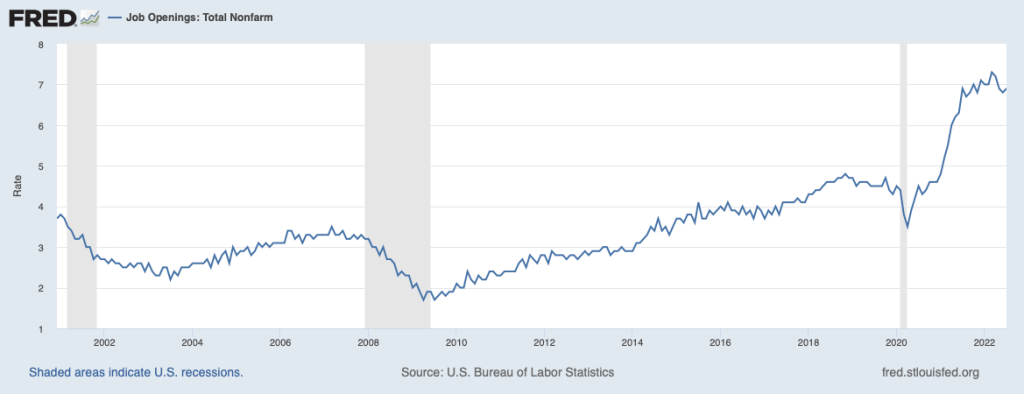
As the following figure shows, the rate of job openings remained very high, even in comparison with the strong labor market of 2019 and early 2020 before the Covid-19 pandemic began disrupting the U.S. economy. The BLS defines a job opening as a full-time or part-time job that a firm is advertising and that will start within 30 days. The rate of job openings is the number of job openings divided by the number of job openings plus the number of employed workers, multiplied by 100.

In the following figure, we compare the total number of job openings to the total number of people unemployed. The figure shows that in July 2022 there were almost two jobs available for each person who was unemployed.

Typically, a strong job market with high rates of job openings indicates that firms are expanding and that they expect their profits to be increasing. As we discuss in Macroeconomics, Chapter 6, Section 6.2 (Microeconomics and Economics, Chapter 8, Section 8.2) the price of a stock is determined by investors’ expectations of the future profitability of the firm issuing the stock. So, we might have expected that on the day the BLS released the July JOLTS report containing good news about the labor market, the stock market indexes like the Dow Jones Industrial Average, the S&P 500, and the Nasdaq Composite Index would rise. In fact, though the indexes fell, with the Dow Jones Industrial Average declining a substantial 300 points. As a column in the Wall Street Journal put it: “A surprisingly tight U.S. labor market is rotten news for stock investors.” Why did good news about the labor market could cause stock prices to decline? The answer is found in investors’ expectations of the effect the news would have on monetary policy.

In August 2022, Fed Chair Jerome Powell and the other members of the Federal Reserve Open Market Committee (FOMC) were in the process of tightening monetary policy to reduce the very high inflation rates the U.S. economy was experiencing. In July 2022, inflation as measured by the percentage change in the consumer price index (CPI) was 8.5 percent. Inflation as measured by the percentage change in the personal consumption expenditures (PCE) price index—which is the measure of inflation that the Fed uses when evaluating whether it is hitting its target of 2 percent annual inflation—was 6.3 percent. (For a discussion of the Fed’s choice of inflation measure, see the Apply the Concept “Should the Fed Worry about the Prices of Food and Gasoline,” in Macroeconomics, chapter 15, Section 15.5 and in Economics, Chapter 25, Section 25.5.)

To slow inflation, the FOMC was increasing its target for the federal funds rate—the interest rate that banks charge each other on overnight loans—which in turn was leading to increases in other interest rates, such as the interest rate on residential mortgage loans. Higher interest rates would slow increases in aggregate demand, thereby slowing price increases. How high would the FOMC increase its target for the federal funds rate? Fed Chair Powell had made clear that the FOMC would monitor economic data for indications that economic activity was slowing. Members of the FOMC were concerned that unless the inflation rate was brought down quickly, the U.S. economy might enter a wage-price spiral in which high inflation rates would lead workers to push for higher wages, which, in turn, would increase firms’ labor costs, leading them to raise prices further, in response to which workers would push for even higher wages, and so on. (We discuss the concept of a wage-price spiral in this earlier blog post.)

In this context, investors interpretated data showing unexpected strength in the economy—particularly in the labor market—as making it likely that the FOMC would need to make larger increases in its target for the federal fund rate. The higher interest rates go, the more likely that the U.S. economy will enter an economic recession. During recessions, as production, income, and employment decline, firms typically experience lower profits or even suffer losses. So, a good JOLTS report could send stock prices falling because news that the labor market was stronger than expected increased the likelihood that the FOMC’s actions would push the economy into a recession, reducing profits. Or as the Wall Street Journal column quoted earlier put it:

“So Tuesday’s [JOLTS] report was good news for workers, but not such good news for stock investors. It made another 0.75-percentage-point rate increase [in the target for the federal funds rate] from the Fed when policy makers meet next month seem increasingly likely, while also strengthening the case that the Fed will keep raising rates well into next year. Stocks sold off sharply following the report’s release.”

Sources: U.S. Bureau of Labor Statistics, “Job Openings and Labor Turnover–July 2022,” bls.gov, August 30, 2022; Justin Lahart, “Why Stocks Got Jolted,” Wall Street Journal, August 30, 2022; Jerome H. Powell, “Monetary Policy and Price Stability,” speech at “Reassessing Constraints on the Economy and Policy,” an economic policy symposium sponsored by the Federal Reserve Bank of Kansas City, Jackson Hole, Wyoming, August 26, 2022; and Federal Reserve Bank of St. Louis.

The Surprisingly Strong Employment Report for January 2022

Leisure and hospitality was one of the industries showing surprisingly strong job growth during January 2022. Photo from the New York Times.

The Bureau of Labor Statistics’ monthly report on the “Employment Situation” is generally considered the best source of information on the current state of the labor market. As we discuss in Macroeconomics, Chapter 9, Section 9.1 (and in Economics, Chapter 19, Section 19.1), economists, policymakers, and investors generally focus more on the establishment survey data on total payroll employment than on the household survey data on the unemployment rate. The initial data on employment from the establishment survey are subject to substantial revisions over time (we discuss this point further below). But the establishment survey has the advantage of being determined by data taken from actual payrolls rather than by unverified answers to survey questions, as is the case with the household survey data. 

The establishment survey data for January 2022 (released on February 4, 2022) showed a surprisingly large increase in employment of 467,000. The consensus forecast had been for a significantly smaller increase of 150,000, with many economists expecting that the data would show a decrease in employment. The establishment survey is collected for pay periods that include the 12th of the month. In January 2022, in many places in the United States that pay period coincided with the height of the wave of infections from the Omicron variant of Covid-19. And, in fact, according to the household survey, the number of people out of work because of illness was 3.6 million in January—the most during the Covid-19 pandemic. So it seemed likely that payroll employment would have declined in January. But despite the difficulties caused by the pandemic, payroll employment increased substantially, likely reflecting firms’ continuing high demand for workers—a demand reflected in the very high level of job openings.

The employment report includes the BLS’s annual data revisions, which are based on a comprehensive payroll count for a particular month in the previous year—in this case, March 2021. The revisions also incorporate changes to the BLS’s seasonal adjustment factors. Each month, the BLS adjusts the raw payroll employment data to reflect seasonal fluctuations such as occur during and after the end-of-year holiday period. For instance, the change from December 2020 to January 2021 in the raw employment data was −2,824,000, whereas the adjusted change was 467,000 (as noted earlier). Obviously this difference is very large and is attributable to the BLS’s seasonal adjustments removing the employment surge in December attributable to seasonal hiring by retail stores, delivery firms, and other businesses strongly affected by the holidays.

The changes to the seasonal adjustment factors made the revisions to the 2021 payroll employment numbers unusually large. For instance, the BLS initially reported that employment increased from June 2021 to July 2021 by 1,091,000, whereas the revision reduced the increase to 689,000. Table A below is reproduced from the BLS report; the figure below the table shows the changes in employment from the previous month as originally published and as revised in the January report. Overall, the BLS revisions now show that employment increased by 217,000 more from 2020 to 2021 than initially estimated. The BLS expressed the opinion that: “Going forward, the updated models should produce more reliable estimates of seasonal movements. [Because there are now] more monthly observations related to the historically large job losses and gains seen in the pandemic-driven recession and recovery, the models can better distinguish normal seasonal movements from underlying trends.”

Source: The BLS “Employment Situation” report can be found here.