Leisure and hospitality was one of the industries showing surprisingly strong job growth during January 2022. Photo from the New York Times.
The Bureau of Labor Statistics’ monthly report on the “Employment Situation” is generally considered the best source of information on the current state of the labor market. As we discuss in Macroeconomics, Chapter 9, Section 9.1 (and in Economics, Chapter 19, Section 19.1), economists, policymakers, and investors generally focus more on the establishment survey data on total payroll employment than on the household survey data on the unemployment rate. The initial data on employment from the establishment survey are subject to substantial revisions over time (we discuss this point further below). But the establishment survey has the advantage of being determined by data taken from actual payrolls rather than by unverified answers to survey questions, as is the case with the household survey data.
The establishment survey data for January 2022 (released on February 4, 2022) showed a surprisingly large increase in employment of 467,000. The consensus forecast had been for a significantly smaller increase of 150,000, with many economists expecting that the data would show a decrease in employment. The establishment survey is collected for pay periods that include the 12th of the month. In January 2022, in many places in the United States that pay period coincided with the height of the wave of infections from the Omicron variant of Covid-19. And, in fact, according to the household survey, the number of people out of work because of illness was 3.6 million in January—the most during the Covid-19 pandemic. So it seemed likely that payroll employment would have declined in January. But despite the difficulties caused by the pandemic, payroll employment increased substantially, likely reflecting firms’ continuing high demand for workers—a demand reflected in the very high level of job openings.
The employment report includes the BLS’s annual data revisions, which are based on a comprehensive payroll count for a particular month in the previous year—in this case, March 2021. The revisions also incorporate changes to the BLS’s seasonal adjustment factors. Each month, the BLS adjusts the raw payroll employment data to reflect seasonal fluctuations such as occur during and after the end-of-year holiday period. For instance, the change from December 2020 to January 2021 in the raw employment data was −2,824,000, whereas the adjusted change was 467,000 (as noted earlier). Obviously this difference is very large and is attributable to the BLS’s seasonal adjustments removing the employment surge in December attributable to seasonal hiring by retail stores, delivery firms, and other businesses strongly affected by the holidays.
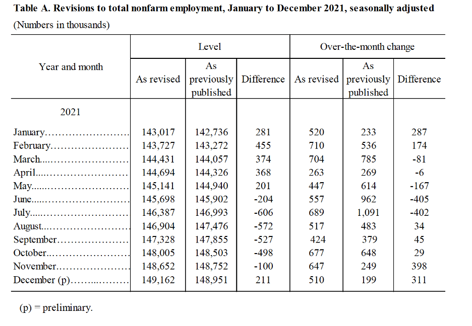
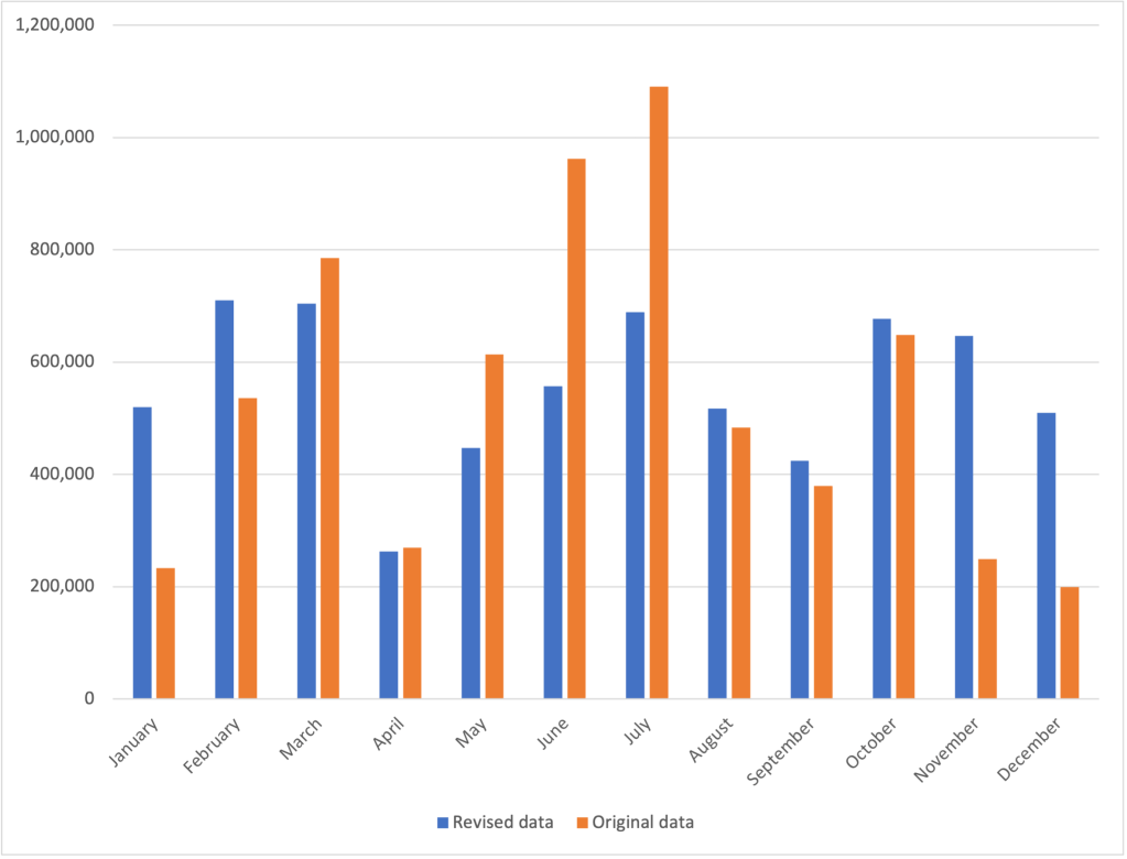
The changes to the seasonal adjustment factors made the revisions to the 2021 payroll employment numbers unusually large. For instance, the BLS initially reported that employment increased from June 2021 to July 2021 by 1,091,000, whereas the revision reduced the increase to 689,000. Table A below is reproduced from the BLS report; the figure below the table shows the changes in employment from the previous month as originally published and as revised in the January report. Overall, the BLS revisions now show that employment increased by 217,000 more from 2020 to 2021 than initially estimated. The BLS expressed the opinion that: “Going forward, the updated models should produce more reliable estimates of seasonal movements. [Because there are now] more monthly observations related to the historically large job losses and gains seen in the pandemic-driven recession and recovery, the models can better distinguish normal seasonal movements from underlying trends.”
Source: The BLS “Employment Situation” report can be found here.
According to the Federal Reserve Act, the Fed must conduct monetary policy “so as to promote effectively the goals of maximum employment, stable prices, and moderate long-term interest rates.” Neither “maximum employment” nor “stable prices” are defined in the act.
The Fed has interpreted “stable prices” to mean a low rate of inflation. Since 2012, the Fed has had an explicit inflation target of 2 percent. When the Fed announced its new monetary policy strategy in August 2020, it modified its inflation target by stating that it would attempt to achieve an average inflation rate of 2 percent over time. As Fed Chair Jerome Powell stated: “Our approach can be described as a flexible form of average inflation targeting.” (Note that although the consumer price index (CPI) is the focus of many media stories on inflation, the Fed’s preferred measure of inflation is changes in the core personal consumption expenditures (PCE) price index. The PCE is a broader measure of the price level than is the CPI because it includes the prices of all the goods and services included in consumption category of GDP. “Core” means that the index excludes food and energy prices. For a further discussion see, Economics, Chapter 25, Section 15.5 and Macroeconomics, Chapter 15, Section 15.5.)
There is more ambiguity about how to determine whether the economy is at maximum employment. For many years, a majority of members of the Federal Open Market Committee (FOMC) focused on the natural rate of unemployment (also called the non-accelerating rate of unemployment (NAIRU)) as the best gauge of when the U.S. economy had attained maximum employment. The lesson many economists and policymakers had taken from the experience of the Great Inflation that lasted from the late 1960s to the early 1980s was if the unemployment rate was persistently below the natural rate of unemployment, inflation would begin to accelerate. Because monetary policy affects the economy with a lag, many policymakers believed it was important for the Fed to react before inflation begins to significantly increase and a higher inflation rate becomes embedded in the economy.
At least until the end of 2018, speeches and other statements by some members of the FOMC indicated that they continued to believe that the Fed should pay close attention to the relationship between the natural rate of unemployment and the actual rate of unemployment. But by that time some members of the FOMC had concluded that their decision to begin raising the target for the federal funds rate in December 2015 and continuing raising it through December 2018 may have been a mistake because their forecasts of the natural rate of unemployment may have been too high. For instance, Atlanta Fed President Raphael Bostic noted in a speech that: “If estimates of the NAIRU are actually too conservative, as many would argue they have been … unemployment could have averaged one to two percentage points lower” than it actually did.
Accordingly, when the Fed announced its new monetary policy strategy in August 2020, it indicated that it would consider a wider range of data—such as the employment-population ratio—when determining whether the labor market had reached maximum employment. At the time, Fed Chair Powell noted that: “the maximum level of employment is not directly measurable and [it] changes over time for reasons unrelated to monetary policy. The significant shifts in estimates of the natural rate of unemployment over the past decade reinforce this point.”
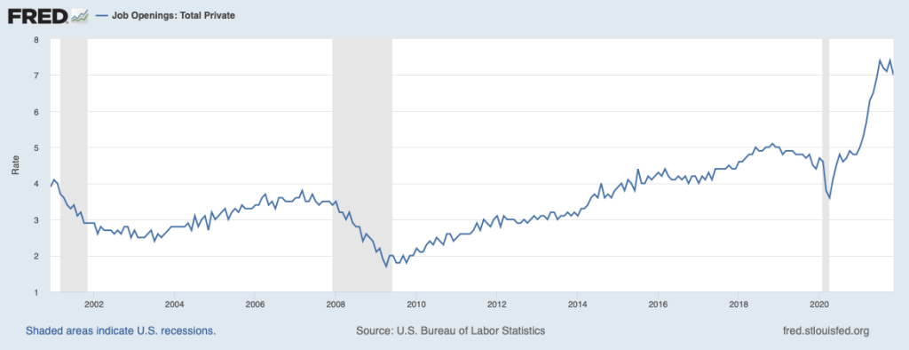
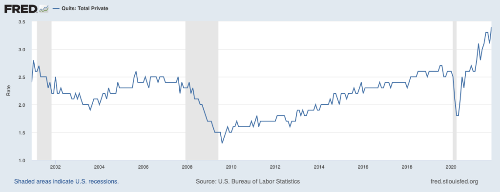
As the economy recovered from the effects of the Covid-19 pandemic, the Fed faced particular difficulty in assessing the state of the labor market. Some labor market indicators appeared to show that the economy was close to maximum employment while other indicators showed that the labor market recovery was not complete. For instance, in December 2021, the unemployment rate was 3.9 percent, slightly below the average of the FOMC members estimates of the natural rate of unemployment, which was 4.0 percent. Similarly, as the first figure below shows, job vacancy rates were very high at the end of 2021. (The BLS calculates job vacancy rates, also called job opening rates, by dividing the number of unfilled job openings by the sum of total employment plus job openings.) As the second figure below shows, job quit rates were also unusually high, indicating that workers saw the job market as being tight enough that if they quit their current job they could find easily another job. (The BLS calculates job quit rates by dividing the number of people quitting jobs by total employment.) By those measures, the labor market seemed close to maximum employment.
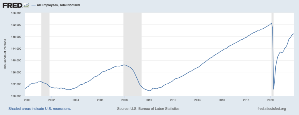
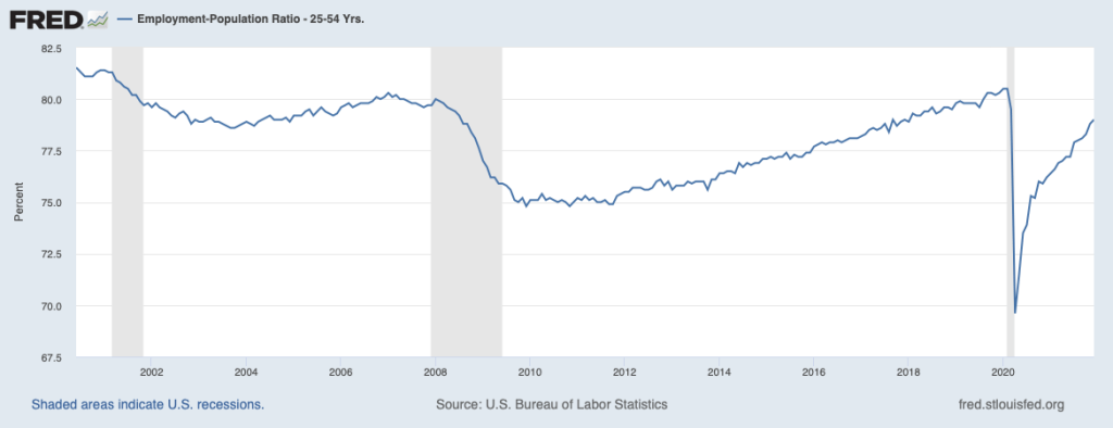
But as the first figure below shows, total employment in December 2021 was still 3.5 million below its level of early 2020, just before the U.S. economy began to experience the effects of the pandemic. Some of the decline in employment can be accounted for by older workers retiring, but as the second figure below indicates, employment of prime-age workers (those between the ages of 25 and 54), had not recovered to pre-pandemic levels.
How to reconcile these conflicting labor market indicators? In January 2022, Fed Chair Powell testified before the Senate Banking Committee as the Senate considered his nomination for a second four-year term as chair. In discussing the state of the economy he offered the opinion that: “We’re very rapidly approaching or at maximum employment.” He noted that inflation as measured by changes in the CPI had been running above 5 percent since June 2021: “If these high levels of inflation get entrenched in our economy, and in people’s thinking, then inevitably that will lead to much tighter monetary policy from us, and it could lead to a recession.” In that sense, “high inflation is a severe threat to the achievement of maximum employment.”
At the time of Powell’s testimony, the FOMC had already announced that it was moving to a less expansionary monetary policy by reducing its purchases of Treasury bonds and mortgage-backed securities and by increasing its target for the federal funds rate in the near future. He argued that these actions would help the Fed achieve its dual mandate by reducing the inflation rate, thereby heading off the need for larger increases in the federal funds rate that might trigger a recession. Avoiding a recession would help achieve the goal of maximum employment.
Powell’s remarks did not make explicit which labor market indicators the Fed would focus on in determining whether the goal of maximum employment had been obtained. It did make clear that the Fed’s new policy of average inflation targeting did not mean that the Fed would accept inflation rates as high as those of the second half of 2021 without raising its target for the federal funds rate. In that sense, the Fed’s monetary policy of 2022 seemed consistent with its decades-long commitment to heading off increases in inflation before they lead to a significant increase in the inflation rate expected by households, businesses, and investors.
Note: For a discussion of the background to Fed policy, see Economics, Chapter 25, Section 25.5 and Chapter 27, Section 17.4, and Macroeconomics, Chapter 15, Section 15.5 and Chapter 17, Section 17.4.
Sources: Jeanna Smialek, “Jerome Powell Says the Fed is Prepared to Raise Rates to Tame Inflation,” New York Times, January 11, 2022; Nick Timiraos, “Fed’s Powell Says Economy No Longer Needs Aggressive Stimulus,” Wall Street Journal, January 11, 2022; and Federal Open Market Committee, “Meeting Calendars, Statements, and Minutes,” federalreserve.gov, January 5, 2022.
During 2020, Congress and President Donald Trump responded to the Covid-19 pandemic with very aggressive fiscal policy initiatives. First, in March 2020, Congress enacted the Coronavirus Aid, Relief, and Economic Security (CARES) Act. The CARES Act increased the federal government’s expenditures by $1.9 trillion. Then, in December 2020, in response to the continuing effects of the pandemic, Congress and President Trump included an additional $915 billion in expenditures related to Covid-19 in the Consolidated Appropriations Act. These two fiscal policy actions included payments directly to households and supplemental unemployment insurance payments. Higher income households were not eligible for the direct payments (often referred to as “stimulus payments”). Higher income households were also less likely to be unemployed and so were less likely to receive the supplemental unemployment insurance payments.
In Chapter 17, Section 17.4, we discuss the unequal distribution of income in the United States. Because the federal payments were targeted toward lower and middle income households, did the payments result in a decline in income inequality? Table 17.6 in Chapter 17, shows a common measure of the distribution of income: Households in the United States are divided into five income quintiles, from the 20 percent with the lowest incomes to the 20 percent with the highest incomes, along with the fraction of total income received by each of the five groups. The following table displays the distribution of income using this measure for 2019 and 2020. (We also include the data for the share of income received by the 5 percent of households with the highest incomes.) Note that the definition of income used in the table includes tax payments households make in that year in addition to payments—including the stimulus payments—received from the government. The income is also “equivalence adjusted,” which means that income is adjusted to account for how many adults and children are in a household.
Year
Lowest 20%
Second 20%
Middle 20%
Fourth 20%
Highest 20%
Highest 5%
2019
4.7%
10.4%
15.7%
22.6%
46.6%
19.9%
2020
5.1%
10.9%
16.0%
22.8%
45.2%
18.9%
Percentage change in income share
8.7%
4.8%
2.1%
0.8%
−3.0%
−5.1%
The table shows that the distribution of income in the United States became somewhat more equal during 2020, with the share of income going to each of the first four quintiles increasing, while the income of the highest quintile declined. The income share of the lowest quintile increased the most—by 8.7 percent—while the income share of the top 5 percent of households decreased by 5.1%. In that section of Chapter 17, we discuss the Gini coefficient, which is a measure of how unequal the distribution of income is. The Gini coefficient ranges between 0 and 1 with higher values indicating a more unequal distribution. Between 2019 and 2020, the Gini coefficient decline from 0.416 to 0.399, or by 4.1 percent, which measure the extent to which the income distribution became more equal.
Will the reduction in income inequality the United States experienced during 2020 persist? It seems likely to, at least through 2021, given that in March 2021, Congress and President Joe Biden enacted the American Rescue Plan, which included payments to households of up to $1,400 per eligible household member. As with the payments to households made during 2020, high-income households were not eligible. Congress also extended supplemental unemployment insurance payments through early September 2021 in states that were willing to accept the payments.
What about after federal stimulus payments to households end? (As of late 2021, it appeared unlikely that Congress and President Biden planned on enacting any further payments.) One indication that some of the reduction in inequality might be sustained comes from the sharp increases in the wages of many low-skilled workers. For instance, in October 2021, the wages (as measured by their average hourly earnings) of workers in the leisure and hospitality industry, which includes workers in restaurants and hotels, increased by nearly 12 percent over the previous year. For all workers in the private sector, wages increased by about 5 percent over the same period. Many of the workers in this industry have low incomes. So, the fact that their wages were increasing more than twice as fast as wages in the overall economy indicates that at least some low-income workers were closing the earnings gap with other workers.
Sources: Emily A. Shrider, Melissa Kollar, Frances Chen, and Jessica Semega, U.S. Census Bureau, Current Population Reports, P60-270, Income and Poverty in the United States: 2020, Washington, DC, U.S. Government Printing Office, September 2021, Table C-3; and U.S. Bureau of Labor Statistics.
As we discuss in Chapter 16, the demand for labor depends on the marginal product of labor. In our basic model of a competitive labor market we assume that all workers have the same ability, skills, and training. Firms can hire as many workers as they would like at the market equilibrium wage. Because, by assumption, all workers have the same abilities, firms don’t have to worry about whether one person might be less able or willing to perform the assigned work than another person.
In reality, we know that most firms face more complicated hiring decisions. Even for a job, such as being a cashier in supermarket, that most people can be quickly trained to do, workers differ in how well they carry out their tasks and whether they can be relied on to regularly show up for work and to treat customers politely.
When hiring workers, firms face a problem of asymmetric information: Workers know more about whether they intend to work hard than firms know. Even for applicants who have a work history, a firm may have difficulty discovering how well or how poorly the applicant performed his or her duties in earlier jobs. In responding to inquiries from other firms about a job applicant, firms are rarely willing to do more than confirm that a person has worked at the firm because they are afraid that reporting anything negative about the person—even if true—might expose the firm to a law suit. In Section 16.5, we discuss the field of personnel economics, which includes the study of how firms design compensation policies that attempt to ensure that workers have an incentive to work hard.
When hiring someone entering the labor market, such as a new college graduate, firms have a particular problem in gauging the likely performance of a worker who may have no job history. In this case, there may not be a problem of asymmetric information because the worker may also be uncertain as to how well he or she will be able to perform the job, particularly if the worker has not previously held a full-time job in that field. When hiring new college graduates, firms may rely on an applicant’s college grades, the reputation of the applicant’s college, and the applicant’s scores on standardized test. Some firms have also developed their own tests to measure an applicant’s cognitive skills, knowledge relevant to the position applied for, and even psychological temperament. Some technology firms and investment banks ask applicants to complete demanding problems that may be unrelated to either technology or banking but can provide insight into whether the applicant has the cognitive ability and temperament to quickly complete complicated tasks.
Teams in the National Football League (NFL) face an interesting problem when hiring new players, particularly those playing the position of quarterback. College football players hoping to play professional football enter the NFL draft in which each of the 32 teams select players in eight rounds, with the selections being in reverse order of the teams’ records during the previous football season. There is often a substantial gap between an athlete’s ability to be successful playing college football and his ability to be successful in the NFL. As a result, many players who are stars in college are unable to succeed as professionals.
The position of quarterback is usually thought to be the most difficult to succeed at. Many highly-regarded college quarterbacks fail to do well in the NFL. Teams typically settle on one player as their starting quarterback who will play most of the time. But teams also have one or two backups. Sometimes the backups are older, former starters on other teams, but often they are players chosen in the draft of college players. It’s very difficult to judge how well a quarterback is likely to perform except by seeing him play in a game. Players who perform well in practice often don’t play well in games. As a result, a backup quarterback may be drafted and, if the starting quarterback on his team remains healthy and is effective, earn a nice salary from year to year without actually playing in many games. If a team’s starting quarterback is injured or is ineffective, the backup quarterback may play in several games during a season.
If the backup shows himself to be an effective player, the team may decide to retain him as the starter—with a substantial increase in salary. But given the difficulty of playing the position of quarterback, a more likely outcome is that the backup plays poorly and the team decides to draft another backup quarterback the following year.
The result is an odd situation: The more that a backup quarterback plays in games, often the less likely he is to keep his job. And the less that a backup quarterback plays, the more likely he is to keep his job. Or as one NFL head coach put it: “Backups who don’t play a lot tend to have long NFL careers, while those who are exposed [by actually] playing … have shorter careers.”
This outcome is an extreme example of the difficulty firms sometimes have in measuring how well new hires are likely to perform in their jobs.
Source for quote: Sportswriter David Lombardi on Twitter, quoting San Francisco 49ers’ head coach Kyle Shanahan, December 14, 2020.
This post on the Federal Reserve Bank of St. Louis’s Page One blog discusses how the belief that automation can lead to permanent job losses is an example of the “lump of labor” fallacy. Click HERE to read the article.
The post refers to the circular-flow diagram, which we discuss in Chapter 2 and in Chapter 18 in the textbook. We discuss the effects of automation and robots on the labor market in Chapter 16.