This yogurt remained the same price although the container shrank from 5.3 ounces to 4.5 ounces.
Each month, hundreds of employees of the Bureau of Labor Statistics (BLS) gather data on prices of goods and services from stores in 87 cities and from websites. The BLS constructs the consumer price index (CPI) by giving each price a weight equal to the fraction of a typical family’s budget spent on that good or service. (CPI is discussed in Macroeconomics, Chapter 9, Section 9.4 and in Economics, Chapter 19, Section 19.4.) Ideally, the BLS tracks prices of the same product over time. But sometimes a particular brand and style of shirt, for example, is discontinued. In that case, the BLS will instead use the price of a shirt that is a very close substitute.
A more difficult problem arises when the price of a good increases at the same time that the quality of the good improves. For instance, a new model iPhone may have both a higher price and a better battery than the model it replaces, so the higher price partly reflects the improvement in the quality of the phone. The BLS has long been aware of this problem and has developed statistical techniques that attempt to identify which part of the price increases are due to increases in quality. Economists differ in their views on how successfully the BLS has dealt with this quality bias to the measured inflation rate. Because of this bias in constructing the CPI, it’s possible that the published values of inflation may overstate the actual annual rate of inflation by 0.5 percentage point. For instance, the BLS might report an inflation rate of 3.5 percent when the actual inflation rate—if the BLS could determine it—was 4.0 percent. As the inflation rate increased beginning in the spring of 2021, a number of observers pointed to hidden inflation that was occurring. There were two main types of hidden inflation:
The quality of some services was declining
Some packaged goods contained smaller quantities at the same price
Here’s one example of the deteriorating quality of some services. Because during 2021 and 2022 many restaurants were having difficulty hiring servers, it was often taking longer for customers to have their orders taken and to have their food brought to the table. Because restaurants were also having difficulty hiring enough cooks, they also limited the items available on their menus. In other words, the service these restaurants were offering was not as good as it had been prior to the pandemic. So even if the restaurants kept their prices unchanged, their customers were paying the same price, but receiving less. Alan Cole, a former senior economist with the Congressional Joint Economic Committee, discussed these other examples on his blog: “hotels clean rooms less frequently on multi-night stays, shipping delays are longer, and phone hold times at airlines are worse.” In a column in the New York Times, economics writer Neil Irwin made similar points: “Complaints have been frequent about the cleanliness of [restaurant] tables, floors and bathrooms.” And: “People trying to buy appliances and other retail goods are waiting longer.”
A column in the Wall Street Journal on business travel by Scott McCartney was headlined “The Incredible Disappearing Hotel Breakfast.” McCartney noted that many hotels continue to advertise free hot breakfasts on their websites and apps but have stopped providing them. He also noted that hotels “have suffered from labor shortages that have made it difficult to supply services such as daily housekeeping or loyalty-group lounges,” in addition to hot breakfasts. In all of these cases, the actual prices of the services had increased more than had the listed prices because the deterioration in quality meant that people were receiving less for their money.
In addition to deterioration in the quality of services, hidden inflation during this period also took the form of consumers buying some packaged goods in which the quantities had been reduced, although the price was unchanged. For example, in June 2022, an article by the Associated Press noted that:
• “A small box of Kleenex now has 60 tissues; a few months ago, it had 65.” • “Chobani Flips yogurts have shrunk from 5.3 ounces to 4.5 ounces.” • “Earth’s Best Organic Sunny Days Snack Bars went from eight bars per box to seven, but the price listed at multiple stores remains $3.69.”
An article in the Wall Street Journal observed that: “Shrinkflation, as economists call it, tends to be easier for companies to pass on to consumers. Despite labels that show price by weight, research shows that most customers look at only the overall price.”
The BLS does try to adjust the measurement of the CPI for shrinkflation, which it can do because the BLS keeps careful track of the quantities included in the packaged goods that are included in its survey.
But the BLS makes no attempt to adjust the CPI for the deterioration in the quality of services because doing so would be very difficult. As Irwin observes: “Customer service preferences—particularly how much good service is worth—varies highly among individuals and is hard to quantify. How much extra would you pay for a fast-food hamburger from a restaurant that cleans its restroom more frequently than the place across the street?” And an economist at the BLS noted that, “We do not capture the decrease in service quality associated with cleaning a [hotel] room every two days rather than one.”
As we noted earlier, most economists believe that the failure of the BLS to fully account for improvements in the quality of goods results in changes in the CPI overstating the true inflation rate. This bias may have been more than offset during 2021–2022 by deterioration in the quality of services resulting in the CPI understating the true inflation rate. As the dislocations caused by the pandemic gradually resolve themselves, it seems likely that the deterioration in services will be reversed. But it’s possible that the deterioration in the provision of some services may persist. Fortunately, unless the deterioration increases over time, it would not continue to distort the measurement of the inflation rate because the same lower level of service would be included in every period’s prices.
Sources: Dee-Ann Durbin, “No, You’re Not Imagining It—Package Sizes Are Shrinking,” apnews.com, June 8, 2022; Annie Gasparro and Gabriel T. Rubin, “The Hidden Ways Companies Raise Prices,” Wall Street Journal, February 12, 2022; Alan Cole, “How I Reluctantly Became an Inflation Crank,” fullstackeconomics.com, September 8, 2021; Scott McCartney, “The Incredible Disappearing Hotel Breakfast—and Other Amenities Travelers Miss,” Wall Street Journal, October 20, 2021; and Neil Irwin, “There Is Shadow Inflation Taking Place All Around Us,” New York Times, October 14, 2021.
To answer the question in the title: Negative supply shocks—shifts to the left in the short-run aggregate supply (SRSAS) curve—and positive demand shocks—shifts to the right in the aggregate demand (AD) curve—both contributed to the acceleration in inflation that began in the spring of 2021. But were the aggregate supply shifts, such as the semiconductor shortage that reduced the supply of new automobiles, more or less important than the aggregate demand shifts, such as the expansionary monetary and fiscal policies?
Adam Hale Shapiro of the Federal Reserve Bank of San Francisco used a basic piece of microeconomic analysis to estimate the contribution of shifts in aggregate supply and shifts in aggregate demand to inflation during this period. He looked at the prices of the more than 100 categories of goods and services in the personal consumption expenditures(PCE) price index. The PCE price index is a measure of the price level similar to the GDP deflator, except it includes only the prices of goods and services from the consumption category of GDP. Changes in the PCE price index are the Federal Reserve’s preferred measure of the inflation rate because that index includes the prices of more goods and services than are included in the consumer price index (CPI).
Shapiro explains how he used microeconomic reasoning to determine whether prices in one of the more than 100 categories of goods and services were increasing because of shifts in supply or because of shifts in demand:
“Shifts in demand move both prices and quantities in the same direction along the upward-sloping supply curve, meaning prices rise as demand increases. Shifts in supply move prices and quantities in opposite directions along the downward-sloping demand curve, meaning prices rise when supplies decline.”
For example, the figure on the left shows the effect on the market for toys of an increase in the demand for toys. (We discuss how shifts in demand and supply curves in a market affect equilibrium price and quantity in Chapter 3, Section 3.4 of Economics, Macroeconomics, and Microeconomics.) The demand curve for toys shifts to the right from D1 to D2, the equilibrium price increases from P1 to P2, and the equilibrium quantity increases from Q1 to Q2. The figure on the right shows the effect on the market for toys if the price increase results from a decrease in the supply of toys rather than from an increase in demand. The supply curve shifts to the left from S1 to S2, the equilibrium price increases from P1 to P2, and the equilibrium quantity decreases from Q1 to Q2.
Shapiro used statistical methods to determine the part of a change in price or quantity that was unexpected. He took this approach in order to focus on short-run changes in these markets caused by shifts in demand and supply rather than long-run changes resulting from “factors such as technological improvements, cost-of-living adjustments to wages, or demographic changes like population aging.” In some cases, the quantity or the price in a market were very close to their expected values, so Shapiro labeled the cause of a price increase in this market as “ambiguous.”
Shapiro notes that: “Categories that experience frequent supply-driven price changes include food and household products such as dishes, linens, and household paper items. Categories that experience frequent demand-driven price changes include motor vehicle-related products, used cars, and electricity.”
The following figure shows Shapiro’s results for the period from January 2020 through April 2022. The height of each column gives the inflation rate in the month measured as the percentage change in the PCE price index from the same month in the previous year. For example, in March 2022, the inflation rate was 6.6 percent. The height of the yellow segment is the part of inflation in that month attributable to increases in demand, the height of the green segment is the part of the inflation in that month that is attributable to decreases in supply, and the height of the green segment is the part of the inflation that Shapiro can’t assign to either demand or supply. In March 2022, increased in demand accounted for 2.2 percentage points of the total 6.6 percentage point increase in inflation. Decreases in supply accounted for 3.3 percentage points, and the remaining 1.2 percentage points had an ambiguous cause.
We can conclude that, measured this way, the increase in inflation from the spring of 2021 through the spring of 2022 was due more to negative supply shocks than to positive demand shocks.
Source: Adam Hale Shapiro, “How Much Do Supply and Demand Drive Inflation?” Federal Reserve Bank of San Francisco Economic Letter, 22-15, June 21, 2022.
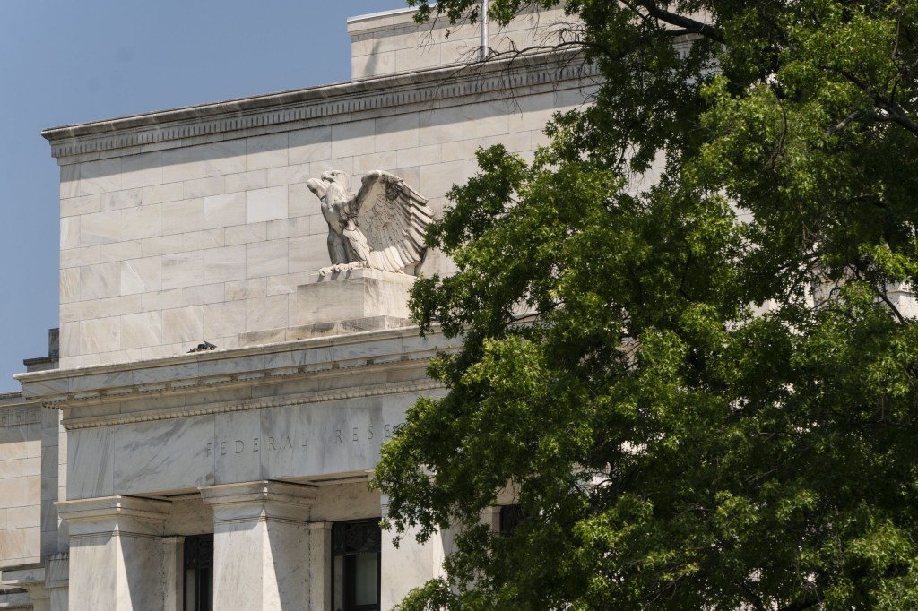
The Federal Reserve building in Washington, DC. Photo from the Wall Street Journal.
Four times per year, the members of the Federal Reserve’s Federal Open Market Committee (FOMC) publish their projections, or forecasts, of the values of the inflation rate, the unemployment, and changes in real gross domestic product (GDP) for the current year, each of the following two years, and for the “longer run.” The following table, released following the FOMC meeting held on March 15 and 16, 2022, shows the forecasts the members made at that time.
Median Forecast
Meidan Forecast
Median Forecast
2022
2023
2024
Longer run
Actual values, March 2022
Change in real GDP
2.8%
2.2%
2.2%
1.8%
3.5%
Unemployment rate
3.5%
3.5%
3.6%
4.0%
3.6%
PCE inflation
4.3%
2.7%
2.3%
2.0%
6.6%
Core PCE inflation
4.1%
2.6%
2.3%
No forecast
5.2%
Recall that PCE refers to the consumption expenditures price index, which includes the prices of goods and services that are in the consumption category of GDP. Fed policymakers prefer using the PCE to measure inflation rather than the consumer price index (CPI) because the PCE includes the prices of more goods and services. The Fed uses the PCE to measure whether it is hitting its target inflation rate of 2 percent. The core PCE index leaves out the prices of food and energy products, including gasoline. The prices of food and energy products tend to fluctuate for reasons that do not affect the overall long-run inflation rate. So Fed policymakers believe that core PCE gives a better measure of the underlying inflation rate. (We discuss the PCE and the CPI in the Apply the Concept “Should the Fed Worry about the Prices of Food and Gasoline?” in Macroeconomics, Chapter 15, Section 15.5 (Economics, Chapter 25, Section 25.5)).
The values in the table are the median forecasts of the FOMC members, meaning that the forecasts of half the members were higher and half were lower. The members do not make a longer run forecast for core PCE. The final column shows the actual values of each variable in March 2022. The values in that column represent the percentage in each variable from the corresponding month (or quarter in the case of real GDP) in the previous year. Links to the FOMC’s economic projections can be found on this page of the Federal Reserve’s web site.
At its March 2022 meeting, the FOMC began increasing its target for the federal funds rate with the expectation that a less expansionary monetary policy would slow the high rates of inflation the U.S. economy was experiencing. Note that in that month, inflation measured by the PCE was running far above the Fed’s target inflation rate of 2 percent.
In raising its target for the federal funds rate and by also allowing its holdings of U.S. Treasury securities and mortgage-backed securities to decline, Fed Chair Jerome Powell and the other members of the FOMC were attempting to achieve a soft landing for the economy. A soft landing occurs when the FOMC is able to reduce the inflation rate without causing the economy to experience a recession. The forecast values in the table are consistent with a soft landing because they show inflation declining towards the Fed’s target rate of 2 percent while the unemployment rate remains below 4 percent—historically, a very low unemployment rate—and the growth rate of real GDP remains positive. By forecasting that real GDP would continue growing while the unemployment rate would remain below 4 percent, the FOMC was forecasting that no recession would occur.
Some economists see an inconsistency in the FOMC’s forecasts of unemployment and inflation as shown in the table. They argued that to bring down the inflation rate as rapidly as the forecasts indicated, the FOMC would have to cause a significant decline in aggregate demand. But if aggregate demand declined significantly, real GDP would either decline or grow very slowly, resulting in the unemployment rising above 4 percent, possibly well above that rate. For instance, writing in the Economist magazine, Jón Steinsson of the University of California, Berkeley, noted that the FOMC’s “combination of forecasts [of inflation and unemployment] has been dubbed the ‘immaculate disinflation’ because inflation is seen as falling rapidly despite a very tight labor market and a [federal funds] rate that is for the most part negative in real terms (i.e., adjusted for inflation).”
Similarly, writing in the Washington Post, Harvard economist and former Treasury secretary Lawrence Summers noted that “over the past 75 years, every time inflation has exceeded 4 percent and unemployment has been below 5 percent, the U.S. economy has gone into recession within two years.”
In an interview in the Financial Times, Olivier Blanchard, senior fellow at the Peterson Institute for International Economics and former chief economist at the International Monetary Fund, agreed. In their forecasts, the FOMC “had unemployment staying at 3.5 percent throughout the next two years, and they also had inflation coming down nicely to two point something. That just will not happen. …. [E]ither we’ll have a lot more inflation if unemployment remains at 3.5 per cent, or we will have higher unemployment for a while if we are actually to inflation down to two point something.”
While all three of these economists believed that unemployment would have to increase if inflation was to be brought down close to the Fed’s 2 percent target, none were certain that a recession would occur.
What might explain the apparent inconsistency in the FOMC’s forecasts of inflation and unemployment? Here are three possibilities:
Fed policymakers are relatively optimistic that the factors causing the surge in inflation—including the economic dislocations due to the Covid-19 pandemic and the Russian invasion of Ukraine and the surge in federal spending in early 2021—are likely to resolve themselves without the unemployment rate having to increase significantly. As Steinsson puts it in discussing this possibility (which he believes to be unlikely) “it is entirely possible that inflation will simply return to target as the disturbances associated with Covid-19 and the war in Ukraine dissipate.”
Fed Chair Powell and other members of the FOMC were convinced that business managers, workers, and investors still expected that the inflation rate would return to 2 percent in the long run. As a result, none of these groups were taking actions that might lead to a wage-price spiral. (We discussed the possibility of a wage-price spiral in earlier blog post.) For instance, at a press conference following the FOMC meeting held on May 3 and 4, 2022, Powell argued that, “And, in fact, inflation expectations [at longer time horizons] come down fairly sharply. Longer-term inflation expectations have been reasonably stable but have moved up to—but only to levels where they were in 2014, by some measures.” If Powell’s assessment was correct that expectations of future inflation remained at about 2 percent, the probability of a soft landing was increased.
We should mention the possibility that at least some members of the FOMC may have expected that the unemployment rate would increase above 4 percent—possibly well above 4 percent—and that the U.S. economy was likely to enter a recession during the coming months. They may, however, have been unwilling to include this expectation in their published forecasts. If members of the FOMC state that a recession is likely, businesses and households may reduce their spending, which by itself could cause a recession to begin.
Sources: Martin Wolf, “Olivier Blanchard: There’s a for Markets to Focus on the Present and Extrapolate It Forever,” ft.com, May 26, 2022; Lawrence Summers, “My Inflation Warnings Have Spurred Questions. Here Are My Answers,” Washington Post, April 5, 2022; Jón Steinsson, “Jón Steinsson Believes That a Painless Disinflation Is No Longer Plausible,” economist.com, May 13, 2022; Federal Open Market Committee, “Summary of Economic Projections,” federalreserve.gov, March 16, 2022; and Federal Open Market Committee, “Transcript of Chair Powell’s Press Conference May 4, 2022,” federalreserve.gov, May 4, 2022.
Emily Mascitis checks prices at an auto-repair shop in Philadelphia. (Photo from the Wall StreetJournal.)
As we discuss in Macroeconomics, Chapter 9, Section 9.4, (Economics, Chapter 19, Section 19.4) in calculating the consumer price index (CPI) each month, the Bureau of Labor Statistics sends hundreds of employees to gather price data from stores and offices. A reporter for the Wall Street Journal followed a price checker as she visited an auto-repair shop, a grocery store, and other businesses.
The article provides an excellent discussion of the care with which prices are collected, particularly with respect to making sure that the prices are for the same good or service each month. For instance, while in a grocery, the price checker almost made the mistake of recording the price of a can of low sodium chicken noodle soup, rather than the price of regular chicken noodle soup as in previous months.
At one point, the price checker noted that the price of clementines had been increasing rapidly and remarked that when buying fruit for her own family “We need to pick a less expensive fruit.” Switching from buying a fruit, in this case clementines, with a price that is increasing rapidly to a fruit with a price that is increasing more slowly, say regular oranges, is an example of the substitution bias. That’s one of the four biases discussed in Section 9.4 that can cause the measured increase in the CPI to overstate the true rate of inflation.
The article can be found here. (A subscription may be required.)
Source: Rachel Wolfe, “How the Inflation Rate Is Measured: 477 Government Workers at Grocery Stores,” Wall Street Journal, May 10, 2022.
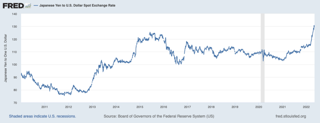
From early March to early May 2022, the Japanese yen persistently lost value versus the U.S. dollar. Between March 1 and May 9, the yen declined by 14% against the dollar, which is a substantial loss in value during such a short time period. What explains the decline in the exchange rate between the yen and the dollar during that time? In Macroeconomics, Chapter 18, Section 18.2 (Economics, Chapter 28, Section 28.2), we saw that the exchange rate between most pairs of currencies fluctuates in response to these factors:
The foreign demand for U.S. goods
U.S. interest rates relative to foreign interest rates
Foreign demand for making direct investments or portfolio investments in the United States
The U.S. demand for foreign goods
Foreign interest rates relative to U.S interest rates
U.S. demand for making direct investments or portfolio investments in other countries
The following figure shows movements in the exchange rate between the yen and the U.S. dollar since 2010. During different periods, the factor that is most important in explaining fluctuations in an exchange rate varies. (Important note: The figure follows the convention of expressing the exchange between the yen and dollar in terms of yen per dollar. Therefore, in the figure, an increase in the exchange rate corresponds to a decrease in the value of the yen versus the dollar because it takes more yen to buy one dollar.)
From early March to early May 2022, the decline in value of the yen versus the dollar was mainly the result of U.S. interest rates increasing relative to Japanese interest rates. As the inflation rate increased rapidly in the spring of 2022, both short-term and long-term interest rates in the United States increased, partly in response to policy actions taken by the Federal Reserve. The Federal Reserve was attempting to increase interest rates in order to raise borrowing costs for households and firms, thereby slowing spending and inflation. Japan was experiencing much lower rates of inflation—well below the Bank of Japan’s 2% annual inflation target—so the BOJ was reluctant to increase interest rates. As a consequence, the gap between the interest rate on 10-year U.S. Treasury notes and the interest rate on 10-year Japanese government bonds had risen to 2.9 percentage points.
Higher U.S. interest rates caused a shift to the right in the demand for dollars in exchange for yen as foreign investors exchanged their yen for dollars in order to buy U.S. Treasury securities and other U.S. financial assets. As we show in Chapter 18, Figure 18.13, an increase in the demand for dollars (holding all other factors constant) increases the equilibrium exchange rate between the yen and the dollar.
What effect does a stronger dollar and a weaker yen have on the two countries’ economies? A weaker yen means that the yen price of imports from the United States will be higher. The higher prices will increase the Japanese inflation rate, but with inflation being low in in the spring of 2022, Japanese policymakers weren’t concerned by this effect. And because the value of U.S. imports is small relative to the size of the Japanese economy, the effect on the inflation rate wouldn’t be large in any case. The dollar price of Japanese exports to the United States will be lower, which should help Japanese firms exporting to the United States.
The effect on the U.S. economy will be the mirror image of the effect on the Japanese economy. The dollar price of Japanese imports being lower will help reduce the U.S. inflation rate, but not to a great extent because the value of Japanese imports is small relative to the size of the U.S. economy. The yen price of U.S. exports to Japan will be higher, which will be bad news for U.S. firms exporting to Japan.
Finally, many banks, other financial firms, and non-financial firms borrow money in dollars. They do so because over time the advantages of borrowing dollars has increased, even for foreign firms that receive most of their revenue in their domestic currency rather than dollars. In particular, the value of the dollar is relatively stable compared with the value of many other currencies. In addition, the Federal Reserve has made available short-term dollar loans to foreign central banks that allow those banks to provide short-term loans to local firms that are having temporary difficulty making dollar payments on their loans. By late 2021, the total amount of dollar loans made outside of the United States had risen to more than $13 trillion. In the spring of 2022, the value of the dollar was rising not just against the Japanese yen but also against many other currencies. The increase was bad news for foreign firms borrowing in U.S. dollars because it would take more of their domestic currency to buy the dollars necessary to make their loans payments. A large and prolonged increase in the value of the U.S. dollar could possibly upset the stability of the international financial system.
Sources: Yuko Takeo and Komaki Ito, “Japan’s Stepped-Up Warnings Fail to Stem Yen’s Slide Past 128,” bloomberg.com, April 19, 2022; Jacky Wong, “Japan Gets a Taste of the Wrong Type of Inflation,” Wall Street Journal, April 1, 2022; Megumi Fujikawa, “Yen Hits Lowest Level Since 2015, and Japan, U.S. Are OK With That,” Wall Street Journal, March 28, 2022; Bank for International Settlements, “BIS International Banking Statistics and Global Liquidity Indicators at End-September 2021,” January 28, 2022; and Federal Reserve Bank of St. Louis.
On Thursday morning, April 28, the Bureau of Economic Analysis (BEA) released its “advance” estimate for the change in real GDP during the first quarter of 2022. As shown in the first line of the following table, somewhat surprisingly, the estimate showed that real GDP had declined by 1.4 percent during the first quarter. The Federal Reserve Bank of Atlanta’s “GDP Now” forecast had indicated that real GDP would increase by 0.4 percent in the first quarter. Earlier in April, the Wall Street Journal’s panel of academic, business, and financial economists had forecast an increase of 1.2 percent. (A subscription may be required to access the forecast data from the Wall Street Journal’s panel.)
Do the data on real GDP from the first quarter of 2022 mean that U.S. economy may already be in recession? Not necessarily, for several reasons:
First, as we note in the Apply the Concept, “Trying to Hit a Moving Target: Making Policy with ‘Real-Time’ Data,” in Macroeconomics, Chapter 15, Section 15.3 (Economics, Chapter 25, Section 25.3): “The GDP data the BEA provides are frequently revised, and the revisions can be large enough that the actual state of the economy can be different for what it at first appears to be.”
Second, even though business writers often define a recession as being at least two consecutive quarters of declining real GDP, the National Bureau of Economic Research has a broader definition: “A recession is a significant decline in activity across the economy, lasting more than a few months, visible in industrial production, employment, real income, and wholesale-retail trade.” Particularly given the volatile movements in real GDP during and after the pandemic, it’s possible that even if real GDP declines during the second quarter of 2022, the NBER might not decide to label the period as being a recession.
Third, and most importantly, there are indications in the underlying data that the U.S. economy performed better during the first quarter of 2022 than the estimate of declining real GDP would indicate. In a blog post in January discussing the BEA’s advance estimate of real GDP during the fourth quarter of 2021, we noted that the majority of the 6.9 percent increase in real GDP that quarter was attributable to inventory accumulation. The earlier table indicates that the same was true during the first quarter of 2022: 60 percent of the decline in real GDP during the quarter was the result of a 0.84 decline in inventory investment.
We don’t know whether the decline in inventories indicates that firms had trouble meeting demand for goods from current inventories or whether they decided to reverse some of the increases in inventories from the previous quarter. With supply chain disruptions continuing as China grapples with another wave of Covid-19, firms may be having difficulty gauging how easily they can replace goods sold from their current inventories. Note the corresponding point that the decline in sales of domestic product (line 2 in the table) was smaller than the decline in real GDP.
The table below shows changes in the components of real GDP. Note the very large decline exports and in purchases of goods and services by the federal government. (Recall from Macroeconomics, Chapter 16, Section 16.1, the distinction between government purchases of goods and services and total government expenditures, which include transfer payments.) The decline in federal defense spending was particularly large. It seems likely from media reports that the escalation of Russia’s invasion of Ukraine will lead Congress and President Biden to increase defense spending.
Notice also that increases in the non-government components of aggregate demand remained fairly strong: personal consumption expenditures increased 2.7 percent, gross private domestic investment increased 2.3 percent, and imports surged by 17.7 percent. These data indicate that private demand in the U.S. economy remains strong.
So, should we conclude that the economy will shrug off the decline in real GDP during the first quarter and expand during the remainder of the year? Unfortunately, there are still clouds on the horizon. First, there are the difficult to predict effects of continuing supply chain problems and of the war in Ukraine. Second, the Federal Reserve has begun tightening monetary policy. Whether Fed Chair Jerome Powell will be able to bring about a soft landing, slowing inflation significantly while not causing a large jump in unemployment, remains the great unknown of economic policy. Finally, if high inflation rates persist, households and firms may respond in ways that are difficult to predict and, may, in particular decide to reduce their spending from the current strong levels.
Adam Smith bronze statue on Royal Mile Market square in front of Saint Gilles Cathedral in Edinburgh, Scotland.
Growth matters. A lot. A slightly higher rate of economic growth, sustained over time, can make the difference between a big increase in living standards and relative stagnation. Whether we can still generate strong and steady growth is a “$64,000 question” for the economy — the question. Nobel Prize–winning economist Robert Lucas famously observed that once economists think of long-term growth, it is hard to think of anything else. A pro-growth policy agenda is a good idea because growth is a good idea.
But a deeper question remains: Is public support for growth guaranteed? Oren Cass of American Compass refers to growth and economists’ fealty to economic participation for all as “economic piety.” This critique resonates for a simple reason: Forces that propel growth invariably leave a wake of economic disruption for people in many places and political disruption for the nation. A serious discussion of pro-growth policy must account for that disruption.
A conventional pro-growth policy agenda can be enhanced by support for openness to markets, ideas, and new ways of doing things, and for the ability of firms to adapt to change. Such an enhanced agenda would center on infrastructure broadly defined, development and dissemination of better management practices, and reduced barriers to competition.
Yet the political process, and even many a conservative, is openly skeptical of such an agenda. This skepticism is rooted not in disagreement over the future of scientific advances or of organizational adaptation — but in a concern that growth’s benefits be shared broadly. Addressing this skepticism head-on is essential for rebuilding social support for growth and for countering well-meaning but potentially harmful policies.
The system that needs defending is a mature and successful one. Adam Smith, the great proponent of the “invisible hand” (not the visible hand of a state-directed economy), saw openness and competition as worth the candle. His 1776 publication of The Wealth of Nations came before what we would recognize today as industrial capitalism, though technological change and globalization were features of economic debates in the aftermath of Smith’s ideas.
Smith’s radical insight is central to economic policy today: National prosperity (the “wealth of a nation”) is represented by consumption of goods and services by its people — i.e., their living standards. The goal of the economy in Smith’s telling was to make the economic pie as large as possible. His advocacy of free markets and competition rested on their ability to boost consumption possibilities.
Two centuries later, Nobel laureates Kenneth Arrow and Gérard Debreu added the jargon and mathematics of contemporary economics to formalize Smith’s intuition. While individuals and firms act independently, competitive markets lead to an efficient allocation of resources and a maximized economic pie. Friedrich Hayek, another Nobel laureate, hailed the virtue of a decentralized competitive price system in maximizing economic activity.
Smith’s radicalism draws from his attack on mercantilism—the economic orthodoxy of the day—which stressed a zero-sum view of trade and state intervention to promote and protect certain firms and industries. (Sound familiar?) His second radical insight was that the “nation” did not mean the sovereign and the well-connected. In Smith’s view, individuals as consumers—all people—were kings. Finally, channeling the sympathetic concern espoused in his earlier classic, The Theory of Moral Sentiments, Smith championed mass participation in the productive economy as a precondition for human flourishing.
It is fair to say that Smith lacked a theory of per capita growth in the economy over time; indeed, he wrote before the massive increase in living standards attendant upon the Industrial Revolution. After 1800, per capita income in the United Kingdom — and the United States — witnessed a 30-fold increase. There have also been major improvements in the quality of goods and services that such a statistic doesn’t quite capture. And, of course, many of today’s offerings — from smartphones to computers to air-conditioning — were not available even in 1900, let alone 1800.
That lacuna in Smith’s theory partly reflects technical difficulties in modeling growth. Higher output can come from growth in inputs such as labor and capital, but what determines their growth? Today’s economists highlight population growth and society’s willingness to work, save, and invest. Still more important is growth in productivity, or the efficiency with which inputs are used to produce goods and services.
Smith’s pin-factory example — in which output rose with the specialization of tasks — links how things are done with the level of productivity. But what factors determine productivity growth over time? Today’s economic analysis focuses on technology and the process of generating ideas. Since economic growth is still crucial for people seemingly marginalized by capitalism, it’s worth asking whether the economic foundations expressed in The Wealth of Nations are still relevant today. Where does growth come from now? And do those sources still require openness and competition?
The short answer is that they do, but to see why, we need to focus on the ideas of two prominent economists after 1800: Edmund Phelps and Deirdre Nansen McCloskey.
Phelps, a Nobel laureate, has done much to connect growth to Smith’s foundational ideas. He starts with Smith’s emphasis on a great many individuals (not the state or privileged firms) searching for new and better ways of doing things. This relentless search produces innovative ideas, processes, and goods that drive growth — but only if the political economy allows openness. Smith’s messy, “bottom up” version of the market therefore puts mass innovation at the heart of economic growth. Phelps’s argument reflects how Smithian societies committed to openness are best able to prosper and promote growth.
This argument has two important applications. The first is to debunk the sometimes fashionable view of secular productivity decline — that we have run short of new things to discover and exploit. The second is to give an answer to economies struggling with growth in a period of structural changes from technology and globalization. Slowdowns in innovation are likely not due to scientific barrenness but to walls against openness and change — that is, fears of disruption.
Phelps’s concern with economic dynamism draws him to Smith’s arguments against mercantilist tinkering in the economy. Like Smith, he worries about the hidden costs of tinkering with competition by blocking change from the outside and by enabling rent-seeking on the inside. These “corporatist” policies — fashionable among some conservatives at present — inevitably embolden vested interests and cronyism, slowing change and growth. Even seemingly small interventions can subtly diminish innovation, a point to which I’ll return.
Yet such a critique must acknowledge the political consequences of disruption. Dynamism is messy. It creates growth in the aggregate, but with many individual losers as well as individual gainers.
McCloskey, an economic historian, has similarly identified the continuous, large-scale, voluntary, and unfocused search for betterment as the source of new ideas that can produce economic growth. She sees this “innovism” as primarily a cultural force, preferring the term to the more familiar “capitalism,” and connects innovism to economic liberalism. Echoing Smith, she emphasizes how an open economy allows individuals—from the moderately to the spectacularly talented—to “have a go.” This economic liberalism allows competition to enshrine liberty and mass flourishing.
In McCloskey’s telling, growth depends on a liberal tolerance and openness to change, which encourage many people to be alert to opportunity. Sustaining that tolerance as structural shifts bring economic misfortune to many individuals, however, requires more than devotion to Smith.
Therein lies the current economic-policy rub. Economists’ theories of growth bring to mind a coin: Sunny descriptions of growth and dynamism are “heads,” and hand-wringing over disruption is “tails.” As I observed earlier, growth is messy. It can push some individuals, firms, and even industries off well-worn and comfortable paths.
But Smith offers more in defense of growth than paeans to laissez-faire. Though he is sometimes caricatured as being anti-government in all cases, Smith was principally opposed to mercantilist privileges for specific businesses and industries and to the governmentalization of social affairs. He wanted government to provide what economists today call “public goods,” such as national defense, the criminal-justice system, and enforcement of property rights and contracts the institutional underpinnings of commerce and trade. He also favored support for infrastructure to keep commerce flowing freely.
But Smith went further: To prepare workers and enrich their lives, he called for government to provide universal education, and he drew a connection between education and liberty as well as work in a free society. But boosting participation in today’s economy—participation that provides support for growth—will require a bit more.
Not surprisingly, political reaction to economic disruption brings about — pardon the econ-speak—a “demand” for and “supply” of policy actions. Job losses, firm failures, and diminished industry fortunes bring about a demand for help, for adaptation. The political process responds with a supply of ideas in one of two forms: walls or bridges. Walls are protections against disruption or change. Bridges, ways to get somewhere or back, prepare individuals for the changed economy and help those whose economic participation has been disrupted reenter the workforce.
Proposals for walls are familiar. They can be physical, of course, but they needn’t be. Conservative populists advocate limits on trade and technology, in order to advance industrial policy. Some progressives advocate universal basic income. All these policies would diminish the prospects for economic advances.
The most prominent sort of wall today is what I call “modern corporatism.” It assumes that Smith was wrong: The “wealth of a nation” lies not in consumption or living standards (and so ultimately in growth) but in jobs, good jobs, even particular good jobs, with good manufacturing jobs the very paradigm. The sort of tinkering with the market that drew Smith’s ire may actually be a necessary way of recentering economic policy on jobs, so the theory goes. Opportunities for work, and for the dignity it can bring, are surely important.
A gentle industrial policy devised by social scientists who are worried about jobs is not the answer. It results in state tinkering for special interests, precisely the kind of thing that prompted Smith’s criticism of mercantilism. Moreover, as University of Chicago economist Luigi Zingales argues in A Capitalism for the People, it risks a vicious cycle: A little bit of tinkering becomes a lot of tinkering—and anyone who cannot justify special privileges is left out, calling into question social support for growth. Nevertheless, industrial policy has caught the attention of elected officials on the right, from Donald Trump to Josh Hawley to Marco Rubio. While national security and the border can be exceptions as concerns, advice from Milton Friedman to the party of Ronald Reagan this is not.
That said, economists’ invocation of Smith as a proponent of let-’er-rip laissez-faire is neither faithful to Smith nor particularly helpful to individuals and communities buffeted by disruption. With today’s rapid and long-lasting technological change and globalization, “having a go” requires support for acquiring new skills when they are needed.
That is why we need more bridges. Bridges take us somewhere and bring us back. The journey to somewhere is about preparation for new opportunities. The journey back is about reconnecting to the productive economy when economic forces beyond our control have knocked us away.
Economic bridges have three features. The first is that they help people overcome a specific challenge on their way to economic flourishing — they don’t provide that outcome directly. The second is that wider society builds the bridge, through private organizations, governments, or public–private partnerships, as globalization and technological change have introduced significant risks that individuals by themselves cannot avoid. The third feature is that they avoid restraints on openness to changes in markets and ideas.
We once did better, much better. During the Civil War, President Abraham Lincoln worked with Congress to pass the Morrill Act, directing resources to the development of land-grant colleges around the country, extending higher education to citizens of modest means, and enabling workers to develop skills for new industries, particularly in manufacturing. As World War II drew to a close, President Franklin D. Roosevelt and Congress came together to enact the G.I. Bill, helping to educate returning troops for a changing economy.
Supporting economic growth and undergirding broad participation in the economy require similarly bold ideas. To begin, community colleges are the logical workhorses of skill development and retraining, and their presence in regional economies makes them attractive partners for employers. Yet community colleges have seen their state-level public support wither. The Biden administration calls for free tuition, which would boost demand but provide no support for community college to offer a practical education and an emphasis on completion. Amy Ganz, Austan Goolsbee, Melissa Kearney, and I proposed an alternative approach based on the land-grant-college model. We proposed a supply-side program of federal grants to strengthen community colleges — contingent on improved degree-completion rates and labor-market outcomes. To further encourage training, the federal government could offer a tax credit to compensate firms for the risk of losing trained workers. It could also increase the earned-income tax credit for workers with or without children.
New ideas are also needed to promote workers’ reentry into the workforce. Personal reemployment accounts, for example, would support dislocated workers and offer them a reemployment bonus if they found a new job within a certain period of time. The “personal” refers to individuals’ choosing from a range of training and support services. Another idea is to beef up support for place-based assistance to areas with stubbornly high rates of long-term nonemployment. Such support could be integrated with an increase in the earned-income tax credit and the supply-side investment in community colleges. Building on the decentralized approach in the land-grant colleges and grants to community colleges, expanded place-based aid would be delivered via flexible block grants encouraging business and employment.
Broad public support required for growth and dynamism requires both bridge-building and a political language that frames it. Growth, opportunity, and participation are good, and we do not need a new economics. But phrases like “transition cost” and “inevitable economic forces” must give way to bridges of preparation and reconnection.
‘Why did nobody see it coming?” a quizzical Queen of England questioned a quorum of economists at the London School of Economics about the global financial crisis as it emerged in late 2008. How could major disruptive forces build up over time and yet escape the attention of experts and leaders?
Of the disruptive structural changes accompanying economic dynamism, one might ask a similar question. Growth matters. But that growth is one side of a coin whose flip side is disruption is known, certainly to economists. Why has our political discourse not emphasized this basic point?
Why did we not see fatigue with change coming among the people who most had to bear its ill effects?
However foolishly, we did not. Some so-called conservatives today have responded by saying that we should limit change. Surely a better response is that we should seek ever more growth by allowing unfettered change, but also facilitate the establishing of ever more connections in a growing economy. That classical-liberal answer has the better place in American conservatism — and in American economic life.
— This essay is sponsored by National Review Institute.Originally published here.
Lawrence Summers (Photo from harvardmagazine.com.)John Cochrane (Photo from hoover.org.)
In several of our blog posts and podcasts, we’ve discussed Lawrence Summers’s forecasts of inflation. Beginning in February 2021, Summers, an economist at Harvard who served as Treasury secretary in the Clinton administration, argued that the United States was likely to experience rates of inflation that would be higher and persist longer than Federal Reserve policymakers were forecasting. In March 2021, the members of the Fed’s Federal Open Market Committee had an average forecast of inflation of 2.4 percent in 2021, falling to 2.0 percent in 2022. (The FOMC projections can be found here.)
In fact, inflation measured by the CPI has been above 5 percent every month since June 2021; the Fed’s preferred measure of inflation—the percentage change in the price index for personal consumption expenditures—has been above 5 percent every month since October 2021. Summers’s forecasts of inflation have turned out to be more accurate than those of the members of the Federal Open Committee.
In this podcast, Summers discusses his analysis of inflation with four scholars from the Hoover Institution, including economist John Cochrane. Summers explains why he came to believe in early 2021 that inflation was likely to be much higher than generally expected, how long he believes high rates of inflation will persist, and whether the Fed is likely to be able to achieve a soft landing by bringing inflation back to its 2 percent target without causing a recession. The first half of the podcast, in particular, should be understandable to students who have completed the monetary and fiscal policy chapters (Macroeconomics, Chapters 15 and 16; Economics, Chapters 25 and 26). Background useful for understanding the podcast discussion of monetary policy during the 1970s can be found in Chapter 17, Sections 17.2 and 17.3.
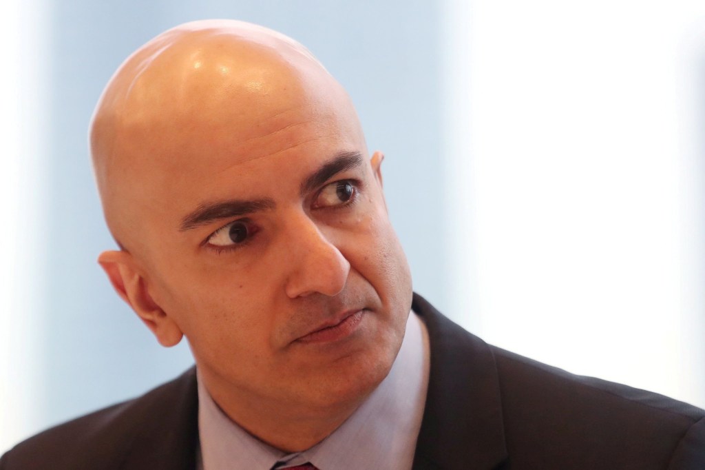
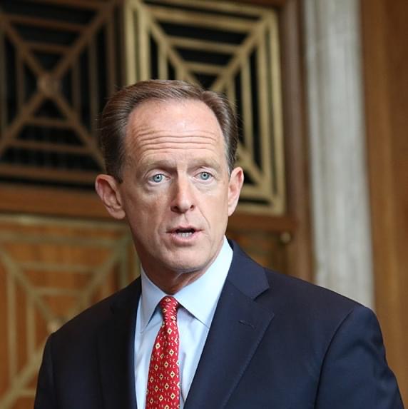
Neel Kashkari, president of the Federal Reserve Bank of Minneapolis. Photo from the Wall Street Journal.Pat Toomey, U.S. Senator from Pennsylvania. Photo from http://www.toomey.senate.gov.
As we discuss in Macroeconomics, Chapter 17, Section 17.4 (Economics, Chapter 27, Section 27.4), the Federal Reserve is unusual among federal government agencies in being able to operate largely independently of Congress and the president. Congress passed the Federal Reserve Act, which established the Federal Reserve System, in 1913, and has amended it several times in the years since. (Note that, as we discuss in the Apply the Concept, “End the Fed?” in this chapter, the U.S. Constitution does not explicitly authorized the federal government to establish a central bank.) Section 2A of the act gives the Federal Reserve System the following charge:
“The Board of Governors of the Federal Reserve System and the Federal Open Market Committee shall maintain long run growth of the monetary and credit aggregates commensurate with the economy’s long run potential to increase production, so as to promote effectively the goals of maximum employment, stable prices, and moderate long-term interest rates.”
Elsewhere in the act, the Fed was given other specified responsibilities, such as supervising commercial banks that are members of the Federal Reserve System and serving on the Financial Stability Oversight Council (FSOC), which is charged with assessing risks to the financial system.
Because Congress can change the structure and operations of the Fed at any time and because Congress has given the Fed only certain specific responsibilities, traditionally the Fed has avoided becoming involved in policy debates that are not directly concerned with its responsibilities. Over the years, most members of the Board of Governors have believed that if the Fed were to become involved in issues beyond monetary policy and the working of the financial system, Congress might decide to revise the Federal Reserve Act to reduce, or even eliminate, Fed independence.
In the spring of 2022, though, there were two instances where some members of Congress argued that the Fed had become involved in policy issues that went beyond the Fed’s responsibilities under the Federal Reserve Act. The first instance involved President Joe Biden’s nomination in January 2022 of Sarah Bloom Raskin to serve on the Fed’s Board of Governors. In 2010, Raskin was nominated to the Board of Governors by President Barack Obama and confirmed by the Senate in a voice vote without significant opposition. (In 2014, she resigned from the Board to accept a position in the Treasury Department.)
Her nomination by President Biden encountered significant opposition, however, largely because in July 2020 she had suggested that when the Fed expanded its lending programs during the Covid-19 pandemic it should have excluded firms in the oil, natural gas, and coal industries: “The Fed is ignoring clear warning signs about the economic repercussions of the impending climate crisis by taking action that will lead to increases in greenhouse gas emissions at a time when even in the short term, fossil fuels are a terrible investment.” Although her supporters argued that in formulating policy the Fed should take into account the threats to financial stability caused by climate change, when it became clear that a majority of the Senate disagreed, Raskin withdrew her nomination.
In April 2022, some members of Congress, including Senator Pat Toomey of Pennsylvania, questioned whether it was appropriate for President Neel Kashkari of the Federal Reserve Bank of Minneapolis to formally support the campaign to amend the Minnesota state constitution to include a provision stating that, “All children have a fundamental right to a quality public education …. It is a paramount duty of the state to ensure quality public schools that fulfill this fundamental right.”
The Bank defended its support for the amendment in a statement on its website: “The Federal Reserve Bank of Minneapolis’ support of the Page amendment is closely linked to the mission of the Federal Reserve. Congress assigned the Federal Reserve the dual goals of achieving (1) stable prices and (2) maximum employment, and one of the greatest determinants of success in the job market is education.”
Senator Toomey strongly disagreed, arguing in a letter of Bank President Kashkari that: “This amendment is highly political, as it wades into an ongoing debate about whether government-run school systems are preferable to parental choice in education.” Toomey asserted that: “These political lobbying efforts by you and other Minneapolis Fed officials … are well beyond the Federal Reserve’s mandate, violate Federal Reserve Bank policies, constitute a misuse of Minneapolis Fed resources, and ultimately undermine the Federal Reserve’s independence and credibility.”
It remains to be seen whether Congress will ultimately accept the arguments of Federal Reserve policymakers such as Kashkari and Raskin that the Fed needs to interpret its mandate from Congress more broadly, or whether Congress will decide to amend the Federal Reserve Act to more explicitly limit the boundaries of Fed action—or to reduce Fed independence in some other ways.
Sources: Sarah Bloom Raskin, “Why Is the Fed Spending So Much Money on a Dying Industry?” New York Times, May 28, 2020; Andrew Ackerman and Ken Thomas, “Sarah Bloom Raskin Withdraws as Biden’s Pick for Top Fed Banking Regulator,” Wall Street Journal, March 15, 2022; Michael S. Derby, “GOP Senator Criticizes Minneapolis Fed Over Education Issue,” Wall Street Journal, April 12, 2022; Federal Reserve Bank of Minneapolis, “Page Amendment: Every Child Deserves a Quality Public Education,” minneapolisfed.org; and Pat Toomey, “Letter to Neel Kashkari,” banking.senate. gov, April 11, 2022.
Authors Glenn Hubbard and Tony O’Brien reconsider the role of inflation in today’s economy. They discuss the Fed’s possible responses by considering responses to similar inflation threats in previous generations – notably the Fed’s response led by Paul Volcker that directly led to the early 1980’s recession. The markets are reflecting stark differences in our collective expectations about what will happen next. Listen to find out more about the Fed’s likely next steps.