Fed Chair Jerome Powell and Fed Vice-Chair Philip Jefferson this summer at the Fed conference in Jackson Hole, Wyoming. (Photo from the AP via the Washington Post.)
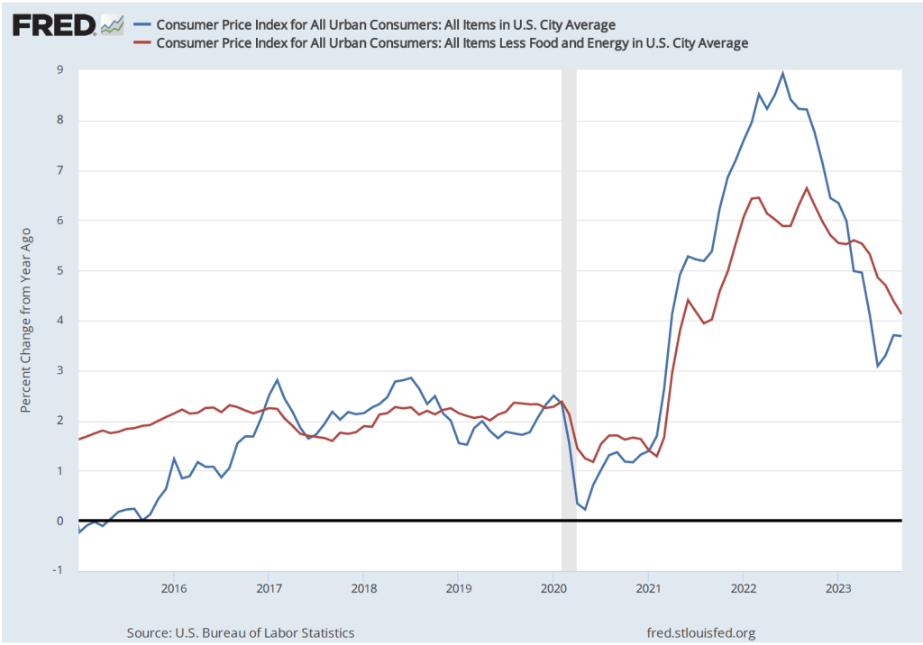
This morning, the Bureau of Labor Statistics (BLS) released its report on the consumer price index (CPI) for September. (The full report can be found here.) The report was consistent with other recent data showing that inflation has declined markedly from its summer 2022 highs, but appears, at least for now, to be stuck in the 3 percent to 4 percent range—well above the Fed’s 2 percent inflation target.
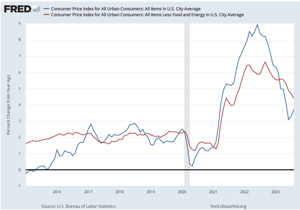
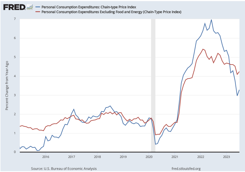
The report indicated that the CPI rose by 0.4 percent in September, which was down from 0.6 percent in August. Measured by the percentage change from the same month in the previous year, the inflation rate was 3.7 percent, the same as in August. Core CPI, which excludes the prices of food and energy, increased by 4.1 percent in September, down from 4.4 percent in August. The following figure shows inflation since 2015 measured by CPI and core CPI.
Reporters Gabriel Rubin and Nick Timiraos, writing in the Wall Street Journal summarized the prevailing interpretation of this report:
“The latest inflation data highlight the risk that without a further slowdown in the economy, inflation might settle around 3%—well below the alarming rates that prompted a series of rapid Federal Reserve rate increases last year but still above the 2% inflation rate that the central bank has set as its target.”
As we discuss in this blog post, some economists and policymakers have argued that the Fed should now declare victory over the high inflation rates of 2022 and accept a 3 percent inflation rate as consistent with Congress’s mandate that the Fed achieve price stability. It seems unlikely that the Fed will follow that course, however. Fed Chair Jerome Powell ruled it out in a speech in August: “It is the Fed’s job to bring inflation down to our 2 percent goal, and we will do so.”
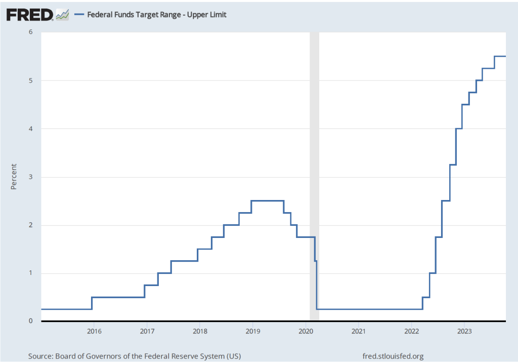
To achieve its goal of bringing inflation back to its 2 percent targer, it seems likely that economic growth in the United States will have to slow, thereby reducing upward pressure on wages and prices. Will this slowing require another increase in the Federal Open Market Committe’s target range for the federal funds rate, which is currently 5.25 to 5.50 percent? The following figure shows changes in the upper bound for the FOMC’s target range since 2015.
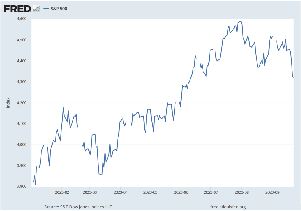
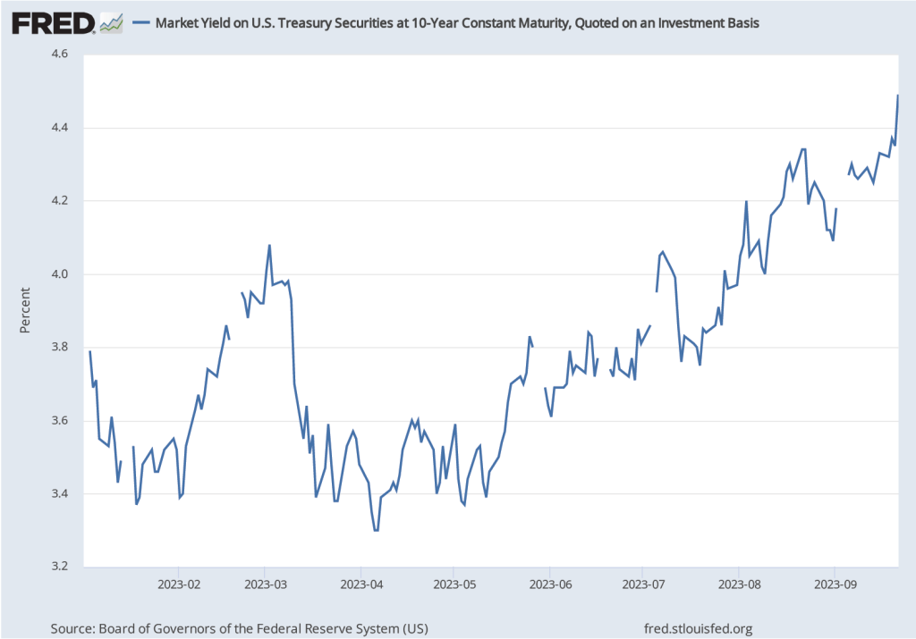
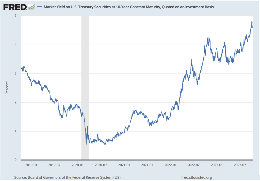
Several members of the FOMC have raised the possibility that financial markets may have already effectively achieved the same degree of policy tightening that would result from raising the target for the federal funds rate. The interest rate on the 10-year Treasury note has been steadily increasing as shown in the following figure. The 10-year Treasury note plays an important role in the financial system, influencing interest rates on mortgages and corporate bonds. In fact, the main way in which monetary policy works is for the FOMC’s increases or decreases in its target for the federal funds rate to result in increases or decreases in long-run interest rates. Higher long-run interest rates typically result in a decline in spending by consumrs on new housing and by businesses on new equipment, factories computers, and software.
Federal Reserve Bank of Dallas President Lorie Logan, who serves on the FOMC, noted in a speech that “If long-term interest rates remain elevated … there may be less need to raise the fed funds rate.” Similarly, Fed Vice-Chair Philip Jefferson stated in a speech that: “I will remain cognizant of the tightening in financial conditions through higher bond yields and will keep that in mind as I assess the future path of policy.”
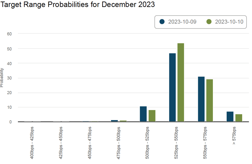
The FOMC has two more meetings scheduled for 2023: One on October 31-November 1 and one on December 12-13. The following figure from the web site of the Federal Reserve Bank of Atlanta shows financial market expectations of the FOMC’s target range for the federal funds rate in December. According to this estimate, financial markets assign a 35 percent probability to the FOMC raising its target for the federal funds rate by 0.25 or more. Following the release of the CPI report, that probability declined from about 38 percent. That change reflects the general expectation that the report didn’t substantially affect the likelihood of the FOMC raising its target for the federal funds rate again by the end of the year.