Supports:Microeconomics, Macroeconomics, Economics, and Essentials of Economics, Chapter 4, Section 4.4
Image generated by ChapGPT
The model of demand and supply is useful in analyzing the effects of tariffs. In Chapter 9, Section 9.4 (Macroeconomics, Chapter 7, Section 7.4) we analyze the situation—for instance, the market for sugar—when U.S. demand is a small fraction of total world demand and when the U.S. both produces the good and imports it.
In this problem, we look at the television market and assume that no domestic firms make televisions. (A few U.S. firms assemble limited numbers of televisions from imported components.) As a result, the supply of televisions consists entirely of imports. Beginning in April, the Trump administration increased tariff rates on imports of televisions from Japan, South Korea, China, and other countries. Tariffs are effectively a tax on imports, so we can use the analysis in Chapter 4, Section 4.4, “The Economic Effect of Taxes” to analyze the effect of tariffs on the market for televisions.
Use a demand and supply graph to illustrate the effect of an increased tariff on imported televisions on the market for televisions in the United States. Be sure that your graph shows any shifts of the curves and the equilibrium price and quantity of televisions before and after the tariff increase.
An article in the Wall Street Journal discussed the effect of tariffs on the market for used goods. Use a second demand and supply graph to show the effect of a tariff on imports of new televisions on the market in the United States for used televisions. Assume that no used televisions are imported and that the supply curve for used televisions is upward sloping.
Solving the Problem Step 1: Review the chapter material. This problem is about the effect of a tariff on an imported good on the domestic market for the good. Because a tariff is a like a tax, you may want to review Chapter 4, Section 4.4, “The Economic Effect of Taxes.”
Step 2: Answer part a. by drawing a demand and supply graph of the market for televisions in the United States that illustrates the effect of an increased tariff on imported televisions. The following figure shows that a tariff causes the supply curve of televisions to shift up from S1 to S2. As a result, the equilibrium price increases from P1 to P2, while the equilibrium quantity falls from Q1 to Q2.
Step 2: Answer part b. by drawing a demand and supply graph of the market for used televisions in the United States that illustrates the effect on that market of an increased tariff on imports of new televisions. Although the tariff on imported televisions doesn’t directly affect the market for used televisions, it does so indirectly. As the article from the Wall Street Journal notes, “Today, in the tariff era, demand for used goods is surging.” Because used televisions are substitutes for new televisions, we would expect that an increase in the price of new televisions would cause the demand curve for used televisions to shift to the right, as shown in the following figure. The result will be that the equilibrium price of used televisions will increase from P1 to P2, while the equilibrium quantity of used televisions will increase from Q1 to Q2.
To summarize: A tariff on imports of new televisions increases the price of both new and used televisions. It decreases the quantity of new televisions sold but increases the quantity of used televisions sold.
In June, the U.S. Census Bureau released its population estimates for 2024. Included was the following graphic showing the change in the U.S. population pyramid from 2004 to 2024. As the graphic shows, people 65 years and older have increased as a fraction of the total population, while children have decreased as a fraction of the total population. (The Census considers everyone 17 and younger to be a child.) Between 2004 and 2024, people 65 and older increased from 12.4 percent of the population to 18.0 percent. People younger than 18 fell from 25.0 percent of the population in 2004 to 21.5 percent in 2024.
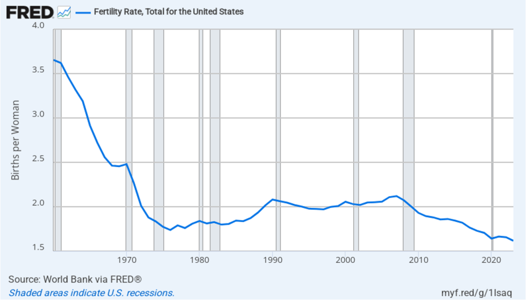
The aging of the U.S. population reflects falling birth rates. Demographers and economists typically measure birth rates as the total fertility rate (TFR), which is defined by the World Bank as: “The number of children that would be born to a woman if she were to live to the end of her childbearing years and bear children in accordance with age-specific fertility rates currently observed.” The TFR has the advantage over the simple birth rate—which is the number of live births per thousand people—because the TFR corrects for the age structure of a country’s female population. Leaving aside the effects of immigration and emigration, a TFR of 2.1 is necessary to keep a country’s population stable. Stated another way, a country needs a TFR of 2.1 to achieve replacement level fertility. A country with a TFR above 2.1 experiences long-run population growth, while a country with a TFR of less than 2.1 experiences long-run population decline.
The following figure shows the TFR for the United States for each year between 1960 and 2023. Since 1971, the TFR has been below 2.1 in every year except for 2006 and 2007. Immigration has helped to offset the effects on population growth of a TFR below 2.1.
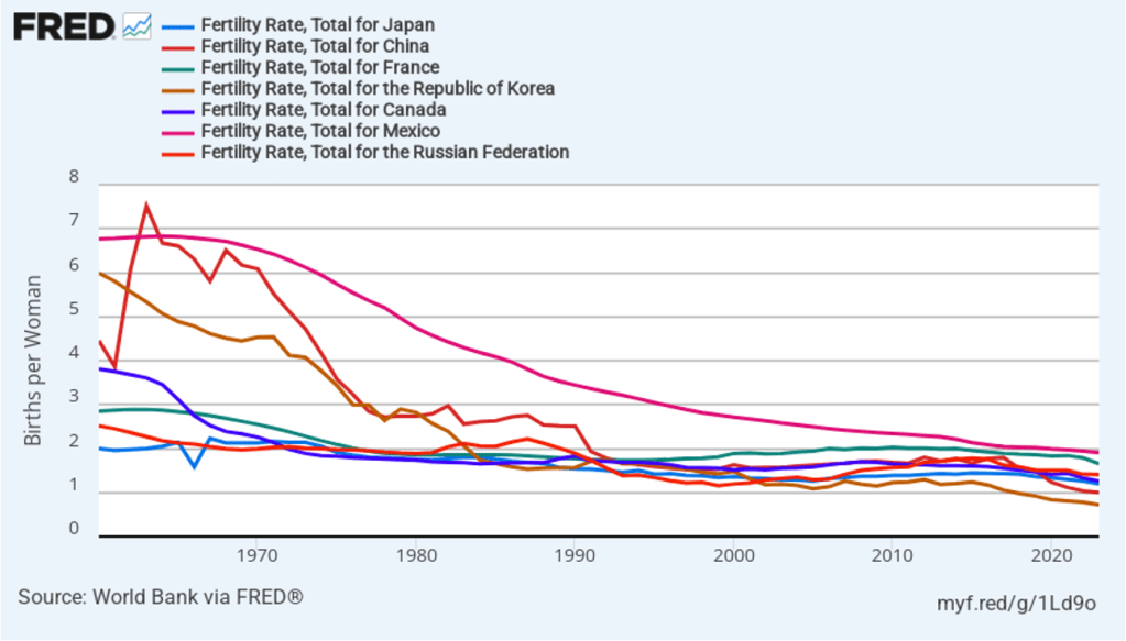
The United States is not alone in experiencing a sharp decline in its TFR since the 1960s. The following figure shows some other countries that currently have below replacement level fertility, including some countries—such as China, Japan, Korea, and Mexico—in which TFRs were well above 5 in the 1960s. In fact, only a relatively few countries, such as Israel and some countries in sub-Saharan Africa are still experiencing above replacement level fertility.
An aging population raises the number of retired people relative to the number of workers, making it difficult for governments to finance pensions and health care for older people. We discuss this problem with respect to the U.S. Social Security and Medicare programs in an Apply the Concept in Macroeconomics, Chapter 16 (Economics, Chapter 26 and Essentials of Economics, Chapter 18). Countries experiencing a declining population typically also experience lower rates of economic growth than do countries with growing populations. Finally, as we discuss in an Apply the Concept in Microeconomics, Chapter 3, different generations often differ in the mix of products they buy. For instance, a declining number of children results in declining demand for diapers, strollers, and toys.
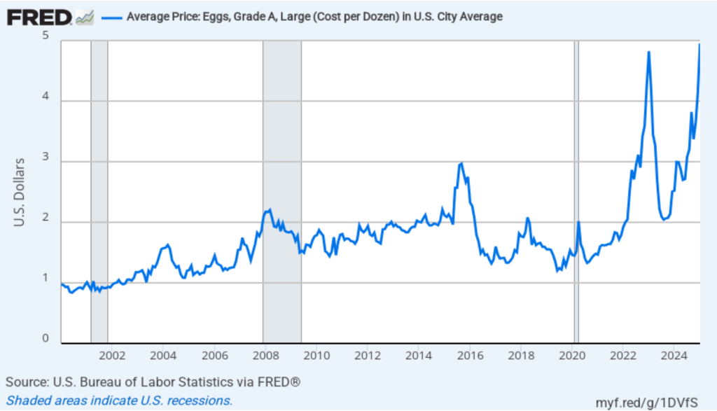
What causes consumer demand for a product to decline? Why does demand for some products suddenly rise? As we discuss in Chapter 3, changes in the relative price of a substitute or a complement cause the demand for a good to shift. For instance, the following figure shows the recent rapid increase in the price of eggs, due in part from the spread of bird flu. We would expect that the increase in the price of eggs will shift to the right the demand curve for egg substitutes, such as the product shown below the figure.
Sometimes a shift in the demand for a product represents a change in consumer tastes. For instance, as we discuss in an Apply the Concept in Chapter 3, for decades most people wore a hat while outdoors. The first photo below shows people walking down a street in New York City in the 1920s. Beginning in the 1960s, hats started to fall out of fashion. As the second photo shows, today few people wear hats—unless they’re walking outside during the winter in the Northeast or the Midwest!
Photo from the New York Daily News
Photo from the New York Times
Technological change can also affect the demand for goods. For example, the development of network television, beginning in the late 1940s, reduced the demand for tickets to movie theaters. Similarly, the development of the internet reduced the demand for physical newspapers.
A recent example of technological change having a substantial effect on a number of consumer goods is the introduction of GLP–1 drugs, beginning in 2005. These drugs, such as Ozempic and Mounjaro, were first developed to treat type 2 diabetes. The drugs were found to significantly reduce appetite in most users, leading to users losing weight. Accordingly, doctors began to prescribe the drugs to treat obesity. By 2025, about half of the users of GLP–1 drugs were doing so to lose weight. A recent article in the Washington Post quoted Jan Hatzius, chief economist at Goldman Sachs, as predicting that by 2028, 60 million people in the United States will be taking a GLP–1 drug.
Many consumers who use these drugs decide to change the mix of foods they eat. Typically, users demand fewer ultra-processed foods, such as chips, cookies, and soft drinks. The percentage of people in the United States who are considered obese—having a body mass index (BMI) of 30 or greater—had been increasing for decades before declining slightly in 2023, the most recent year with available data. It seems likely that the increasing use of GLP–1 drugs helps to explain the decline in obesity.
People taking these drugs have also typically increased the share of foods they eat with higher levels of protein and fiber. These changes in diet are likely to lead to improved health, reducing the demand for some medical services. The number of people experiencing significant weight loss has already begun to reduce demand for extra-large clothing sizes and increase the demand for medium clothing sizes.
How much has the use of Ozempic and similar drugs reduced the demand for snacks? A recent study by Sylvia Hristakeva and Jura Liaukonyt of Cornell University and Leo Feler of Numerator, a market research firm, presents numerical estimates of changes in demand for different foods by users of GLP–1 drugs. The authors assembled a representative sample of 150,000 U.S. households and the households’ grocery purchases from July 2022 through September 2024. They estimate that the share of the U.S. population using a GLP–1 drug increased from 5.5% in October 2023 to 8.8% in July 2024.
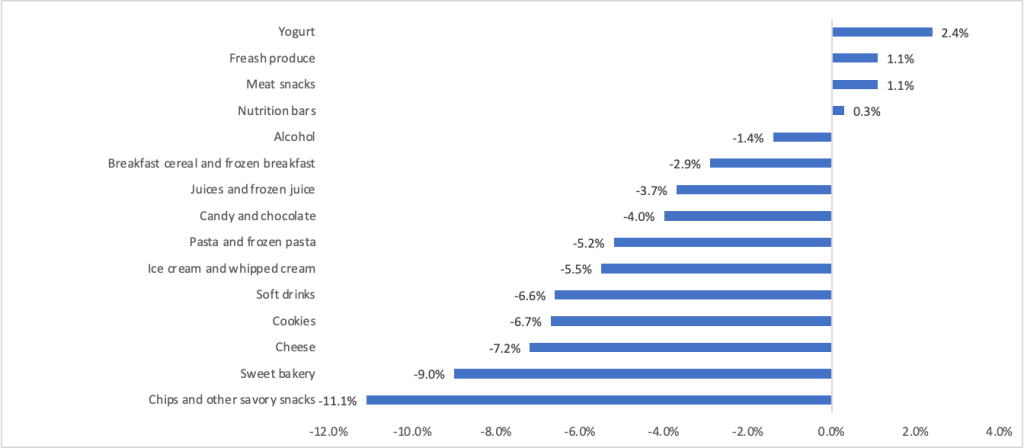
The study finds that households with at least one person using a GLP–1 drug reduced their total grocery shopping by 5.5 percent or $416. The study gathered data on changes in the categories of food that households were buying six months after at least one person in the household began using one of these drugs. The figure below is compiled from data in the study.
As expected, purchases of snacks declined. The category of “chips and other savor snacks” (bottom row in the figure) declined by more than 11 percent. Purchases of sweet bakery products, cheese, cookies, soft drinks, ice cream, and pasta all declined by more than 5 percent. Purchases of yogurt, fresh produce, meat snacks, and nutrition bars, all increased. An article in the Wall Street Journal noted that “food makers are starting to understand better and cater to, in some cases with products specifically designed for” users of this drug. The image below shows some of the new products that Nestle—a major candy producer—has introduced to appeal to users of GLP–1 drugs. Nestle’s Vital Pursuit line of frozen packaged foods contain high levels of protein and fiber.
It’s too early to gauge the full effects of GLP–1 drugs on consumer demand. But it’s already clear that GLP–1 drugs are a striking example of technological change affecting demand in a major industry
Supports: Macroeconomics, Microeconomics, Economics, and Essentials of Economics, Chapter 3, Section 3.1.
Photo from theathletic.com
Caitlin Clark had a sensational college career at the University of Iowa, being named National Player of the Year in her junior and senior years. She was chosen first by the Indiana Fever in the 2024 Women’s National Basketball Association (WNBA) draft of college players. Her popularity drew large crowds to both her home and away games during the 2024 season.
In 2023, the Indiana Fever sold an average of 4,067 tickets to its home games. In 2024, with Clark on the team, the Fever sold an average of 17,036 to its home games. The average price the Fever charged per ticket increased from $60 in 2023 to $110 in 2024. As an article on theathletic.com put it: “Despite the higher price point, even more tickets were sold [by the Fever] this year.”
Can we conclude from this information that Caitlin Clark is so popular that the demance curve for Fever tickets is upward sloping? Briefly explain.
Solving the Problem Step 1: Review the chapter material. This problem is about the effect of a price change on the quantity demand of a good or service, so you may want to review Chapter 3, Section 3.1, “The Demand Side of the Market.”
Step 2: Answer the question by explaining whether it’s likely that the demand curve for tickets to Fever games is upward sloping. It’s unlikely that the demand curve for tickets to Fever games is upward sloping. The law of demand states that, holding everything else constant, when the price of a product rises, the quantity demanded of the product will decrease. When the Fever raised ticket prices from $60 in 2023 to $100 in 2024, we would expect the result to be a movement up the demand curve for tickets, resulting in fewer tickets sold, provided that everything else that would affect the demand for tickets was constant between 2023 and 2024. But everything wasn’t constant because the Fever had Clark on the team in 2024 but not in 2023. Her popularity increased the demand for tickets, shifting the demand curve to the right. In other words, the shift in demand allowed the Fever to sell more tickets at a higher price—moving from a price of $60 and a quantity of 4,067 on the 2023 demand curve to a price of $110 and a quantity of 17,036 on the 2024 demand curve.
Supports:Microeconomics, Chapter 6, Section 6.3, Economics, Chapter 6, Section 6.3, and Essentials of Economics, Chapter 7, Section 7.7.
In August 2023, an article in the Wall Street Journal discussed the effort of the German government to reduce tobacco use. As part of the effort, the government increased the tax on tobacco products, including cigars and cigarettes. The tax increase took effect on January 1, 2022. According to German government data, during 2022 the quantity of cigars and cigarettes sold declined by 8.3 percent. At the same time, the tax revenue the government collected from the tobacco tax declined from €14.7 billion to €14.2 billion.
From this information, can you determine whether the tobacco tax raised the price of cigars and cigarettes by more or less than 8.3 percent? Can you determine whether the demand for cigars and cigarettes in Germany is price elastic or price inelastic? Briefly explain.
According to the Wall Street Journal article, in addition to increasing the tax on tobacco products, the German government took other steps, including banning outdoor advertising of tobacco products, to discourage smoking. Does this additional information affect your answer to parts a.? Briefly explain.
Solving the Problem
Step 1: Review the chapter material. This problem is about the effect of price changes on revenue, so you may want to review Microeconomics, Chapter 6, Section 6.3, “The Relationship between Price Elasticity of Demand and Total Revenue,” or the corresponding sections in Economics, Chapter 6 or Essentials of Economics, Chapter 7.
Step 2:Answer part a. by explaining whether you can tell if the tobacco tax raised the price of cigars and cigarettes by more than 8.3 percent and whether the demand for cigars and cigarettes in Germany is price elastic or price inelastic. We have two pieces of information: (1) In 2022, the quantity of cigars and cigarettes sold in Germany fell by 8.3 percent, and (2) the revenue the German government collected from the tobacco tax fell. We know that if a company increases the price of its product and the total revenue it earns falls, then the demand for the product must be price elastic. We can apply that same reasoning to a government increasing a tax. If the tax increase leads to a fall in revenue we can conclude that the demand for the good being taxed (in this case cigars and cigarettes) is price elastic. When the demand for a good is price elastic, the percentage change in the quantity demanded resulting from a price increase will be greater than the percentage change in the price. Therefore, the percentage change in price resulting from the tax must be less than 8.3 percent. An important qualification to this conclusion is that it holds only if no variable, other than the increase in the tax, affected the demand for cigars and cigarettes during 2022.
Step 3: Answer part b. by explaining how the German government’s banning of outdoor advertising of tobacco products affects your answer to part a. Banning outdoor advertising of tobacco products may have reduced the demand for cigars and cigarettes. If the demand curve for cigars and cigarettes shifted to left, then some of the 8.3 percent decline in the quantity sold may have been the result of the shift in demand rather than the result of the increase in the tax. In other words, the German market for cigars and cigarettes in 2022 may have experienced both a decrease in demand—as the demand curve shifted to the left—and a decrease in the quantity demanded—as the tax increase raised the price of cigars and cigarettes. Given this new information, we can’t be sure that our conclusions in part a.—that the demand for cigars and cigarettes is price elastic and that the tax resulted in an increase in the price of less than 8.3 percent—are correct.
Extra credit: This discussion indicates that in practice economists have to use statistical methods when they estimate the price elasticity of demand for a good or service. The statistical methods make it possible to distinguish the effect of a movement along a demand curve as the price changes from a shift in the demand curve caused by changes in other economic variables.
Sources: Jimmy Vielkind, “Smoking Is a Dying Habit. Not in Germany,” Wall Street Journal, August 31, 2023; and Statistisches Bundesamt, “Taxation of Tobacco Products (Cigarettes, Cigars/Cigarillos, Fine-Cut Tobacco, Pipe Tobacco): Germany, Years, Tax Stamps,” September 10, 2023.
Supports: Microeconomics, Chapter 6, Section 6.3, Economics, Chapter 6, Section 6.3, and Essentials of Economics, Chapter 7, Section 7.7
The Walt Disney Studios in Burbank, California (Photo from reuters.com)
On August 9, Disney released its earnings for the third quarter of its fiscal year. In a conference call with investors, Disney CEO Bob Iger announced that the price for a subscription to the Disney+ streaming service would increase from $10.99 per month to $13.99. An article in the Wall Street Journal quoted Iger as saying that the company had been more uncertain about pricing Disney+ than rival Netflix was about pricing its streaming service “because we’re new at all this.” According to the article, Iger had also said that “there was room to raise prices further [for Disney+] without reducing demand.” A column in the New York Times made the following observation: “The strategy now is to extract more money from subscribers via hefty price increases for Disney+, and hoping that those efforts don’t drive them away.”
a. What is Disney assuming about the price elasticity of demand for Disney+? Briefly explain.
b. Assuming that Disney is only concerned with the total revenue it earns from Disney+, what is the largest percentage of subscribers Disney can afford to “drive away” as a result of its price increase?
c. Why would Iger point out that Disney was new at selling streaming services when discussing the large price increase they were implementing?
d. According to the Wall Street Journal’s account of Iger’s remarks, did he use the phrase “reducing demand” as an economist would? Briefly explain.
Solving the Problem
Step 1: Review the chapter material. This problem is about the effect of a price change on a firm’s revenue, so you may want to review the section “The Relationship between Price Elasticity of Demand and Total Revenue.”
Step 2: Answer part (a) by explaining what Disney is assuming about the price elasticity of demand for Disney+.Disney must be assuming that the demand for Disney+ is price inelastic because they expect that the price increase will increase the revenue they earn from the service. If the demand were price elastic, they would earn less revenue following the price increase.
Step 3: Answer part (b) by calculating the largest percentage of subscribers that Disney can drive away with the price increase. Disney is increasing the price of Disney+ by $3 per month, from $10.99 to $13.99. That is a ($3/$10.99) × 100 = 27.3 percent increase. (Note that we would get a somewhat different result if we used the midpoint formula described in Section 6.1.) For the price increase to increase Disney’s revenue from Disney+, the percentage decrease in the quantity demanded must be less than the percentage increase in the price. Therefore, the price increase can’t drive away more than 27.3 percent of Disney+ subscribers.
Step 4: Answer part (c) by explaining why Iger mentioned that Disney was new to streaming when discussing the Disney+ price increase. Firms sometimes attempt to statistically estimate their demand curves to determine the price elasticity. But particularly when a firm has only recently started selling a product, it often searches for the profit maximizing price through a process of trial and error. Iger contrasted Disney’s relative lack of experience in selling streaming services with Netflix’s much longer experience. In that context, it’s plausible that Disney had been substantially overestimating the price elasticity of demand for Disney+ (that is, Disney had thought that in absolute value, the price elasticity was larger than it actually was). So, the profit maximizing price might be significantly higher than the company had initially thought.
Step 5: Answer part (d) by explaining whether Iger used the phrase “reducing demand” as an economist would. Following a price increase, Disney will experience a reduction in the quantity demanded of Disney+ subscriptions—a movement along the demand curve for subscriptions. For Disney to experience reduced demand for Disney+ subscriptions—a shift of the demand curve—a change in some variable other than price would have to cause consumers to reduce their willingness to buy subscriptions at every price.
Sources: Robbie Whelan, “Disney to Significantly Raise Prices of Disney+, Hulu Streaming Services,” Wall Street Journal, August 9, 2023; and Andrew Ross Sorkin, Ravi Mattu, Sarah Kessler, Michael J. de la Merced, and Ephrat Livni, “Bob Iger Tweaks Disney’s Strategy on Streaming,” New York Times, August 10, 2023.
Inflation as measured by the percentage change in the consumer price index (CPI) from the same month in the previous year was 7.9 percent in February 2022, the highest rate since January 1982—near the end of the Great Inflation that began in the late 1960s. The following figure shows inflation in the new motor vehicle component of the CPI. The 12.4 percent increase in new car prices was the largest since April 1975.
The increase in new car prices was being driven partly by increases in aggregate demand resulting from the highly expansionary monetary and fiscal policies enacted in response to the economic disruptions caused by the Covid-19 pandemic, and partly from shortages of semiconductors and some other car components, which reduced the supply of new cars.
As the following figure shows, inflation in used car prices was even greater. With the exception of June and July of 2021, the 41.2 percent increase in used car prices in February 2022 was the largest since the Bureau of Labor Statistics began publishing these data in 1954.
Because used cars are a substitute of new cars, rising prices of new cars caused an increase in demand for used cars. In addition, the supply of used cars was reduced because car rental firms, such as Enterprise and Hertz, had purchased fewer new cars during the worst of the pandemic and so had fewer used cars to sell to used car dealers. Increased demand and reduced supply resulted in the sharp increase in the price of used cars.
Another factor increasing the prices consumers were paying for cars was a reduction in bargaining—or haggling—over car prices. Traditionally, most goods and services are sold at a fixed price. For example, some buying a refrigerator usually pays the posted price charged by Best Buy, Lowes, or another retailer. But houses and cars have been an exception, with buyers often negotiating prices that are lower than the seller was asking.
In the case of automobiles, by federal law, the price of a new car has to be posted on the car’s window. The posted price is called the Manufacturer’s Suggested Retail Price (MSRP), often referred to as the sticker price. Typically, the sticker price represents a ceiling on what a consumer is likely to pay, with many—but not all—buyers negotiating for a lower price. Some people dislike the idea of bargaining over the price of a car, particularly if they get drawn into long negotiations at a car dealership. These buyers are likely to pay the sticker price or something very close to it.
As a result, car dealers have an opportunity to practice price discrimination: They charge buyers whose demand for cars is more price elastic lower prices and buyers whose demand is less price elastic higher prices. The car dealers are able to separate the two groups on the basis of the buyers willingness to haggle over the price of a car. (We discuss price discrimination in Microeconomics and Economics, Chapter 15, Section 15.5.) Prior to the Covid-19 pandemic, the ability of car dealers to practice this form of price discrimination had been eroded by the availability of online car buying services, such as Consumer Reports’ “Build & Buy Service,” which allow buyers to compare competing price offers from local car dealers. There aren’t sufficient data to determine whether using an online buying service results in prices as low as those obtained by buyers willing to haggle over price face-to-face with salespeople in dealerships.
In any event, in 2022 most car buyers were faced with a different situation: Rather than serving as a ceiling on the price, the MSRP, had become a floor. That is, many buyers found that given the reduced supply of new cars, they had to pay more than the MSRP. As one buyer quoted in a Wall Street Journal article put it: “The rules have changed so dramatically…. [T]he dealer’s position is ‘This is kind of a take-it-or-leave-it proposition.’” According to the website Edmunds.com, in January 2021, only about 3 percent of cars were sold in the United States for prices above MSRP, but in January 2022, 82 percent were.
Car manufacturers are opposed to dealers charging prices higher than the MSRP, fearing that doing so will damage the car’s brand. But car manufacturers don’t own the dealerships that sell their cars. The dealerships are independently owned businesses, a situation that dates back to the beginning of the car industry in the early 1900s. Early automobile manufacturers, such as Henry Ford, couldn’t raise sufficient funds to buy and operate a nationwide network of car dealerships. The manufacturers often even had trouble financing the working capital—or the funds used to finance the daily operations of the firm—to buy components from suppliers, pay workers, and cover the other costs of manufacturing automobiles.
The manufacturers solved both problems by relying on a network of independent dealerships that would be given franchises to be the exclusive sellers of a manufacturer’s brand of cars in a given area. The local businesspeople who owned the dealerships raised funds locally, often from commercial banks. Manufacturers generally paid their suppliers 30 to 90 days after receiving shipments of components, while requiring their dealers to pay a deposit on the cars they ordered and to pay the balance due at the time the cars were delivered to the dealers. One historian of the automobile industry described the process:
The great demand for automobiles and the large profits available for [dealers], in the early days of the industry … enabled the producers to exact substantial advance deposits of cash for all orders and to require cash payment upon delivery of the vehicles …. The suppliers of parts and materials, on the other hand, extended book-account credit of thirty to ninety days. Thus the automobile producer had a month or more in which to assemble and sell his vehicles before the bills from suppliers became due; and much of his labor costs could be paid from dealers’ deposits.
The franchise system had some drawbacks for car manufacturers, however. A car dealership benefits from the reputation of the manufacturer whose cars it sells, but it has an incentive to free ride on that reputation. That is, if a local dealer can take an action—such as selling cars above the MSRP—that raises its profit, it has an incentive to do so even if the action damages the reputation of Ford, General Motors, or whichever firm’s cars the dealer is selling. Car manufacturers have long been aware of the problem of car dealers free riding on the manufacturer’s reputation. For instance, in the 1920s, Ford sent so-called road men to inspect Ford dealers to check that they had clean, well-lighted showrooms and competent repair shops in order to make sure the dealerships weren’t damaging Ford’s brand.
As we discuss in Microeconomics and Economics, Chapter 10, Section 10.3, consumers often believe it’s unfair of a firm to raise prices—such as a hardware store raising the prices of shovels after a snowstorm—when the increases aren’t the result of increases in the firm’s costs. Knowing that many consumers have this view, car manufacturers in 2022 wanted their dealers not to sell cars for prices above the MSRP. As an article in the Wall Street Journal put it: “Historically, car companies have said they disapprove of their dealers charging above MSRP, saying it can reflect poorly on the brand and alienate customers.”
But the car manufacturers ran into another consequence of the franchise system. Using a franchise system rather than selling cars through manufacturer owned dealerships means that there are thousands of independent car dealers in the United States. The number of dealers makes them an effective lobbying force with state governments. As a result, most states have passed state franchise laws that limit the ability of car manufacturers to control the actions of their dealers and sometimes prohibit car manufacturers from selling cars directly to consumers. Although Tesla has attained the right in some states to sell directly to consumers without using franchised dealers, Ford, General Motors, and other manufacturers still rely exclusively on dealers. The result is that car manufacturers can’t legally set the prices that their dealerships charge.
Will the situation of most people paying the sticker price—or more—for cars persist after the current supply chain problems are resolved? AutoNation is the largest chain of car dealerships in the United States. Recently, Mike Manley, the firm’s CEO, argued that the substantial discounts from the sticker price that were common before the pandemic are a thing of the past. He argued that car manufacturers were likely to keep production of new cars more closely in balance with consumer demand, reducing the number of cars dealers keep in inventory on their lots: “We will not return to excessively high inventory levels that depress new-vehicle margins.”
Only time will tell whether the situation facing car buyers in 2022 of having to pay prices above the MSRP will persist.
Sources: Mike Colias and Nora Eckert, “A New Brand of Sticker Shock Hits the Car Market,” Wall Street Journal, February 26, 2022; Nora Eckert and Mike Colias, “Ford and GM Warn Dealers to Stop Charging So Much for New Cars,” Wall Street Journal, February 9, 2022; Gabrielle Coppola, “Car Discounts Aren’t Coming Back After Pandemic, AutoNation Says,” bloomberg.com, February 9, 2022; cr.org/buildandbuy; Lawrence H. Seltzer, A Financial History of the American Automobile Industry, Boston: Houghton-Mifflin, 1928; and Federal Reserve Bank of St. Louis.
Authors Glenn Hubbard and Tony O’Brien as they talk about the leading economic issue of early 2022 – inflation! They discuss the resurgence of inflation to levels not seen in 40 years due to a combination of miscalculations in monetary and fiscal policy. The role of Quantitative Easing (QE) – and its future – is discussed in depth. Listen today to gain insights into the economic landscape.
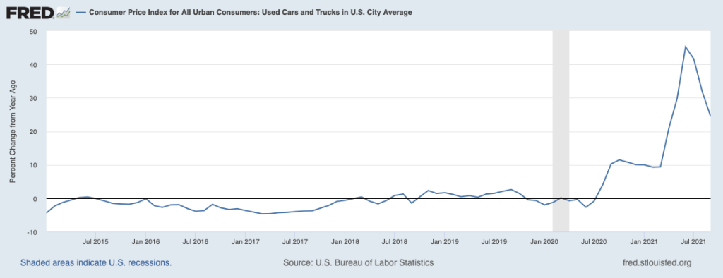
The term “sticker shock” was first used during the 1970s to describe the surprise car buyers experienced when seeing how much car prices had risen. Because inflation during that decade was so high, anyone who hadn’t bought a car for several years was unprepared for the jump in car prices. During 2020 and 2021, sticker shock returned, particularly to the used car market. Prices were increasing so rapidly that even people who had purchased a car a year or two before were surprised by the increases.
The following graph shows U.S. Bureau of Labor Statistics (BLS) data on inflation in the market for used cars in the months since January 2015. Inflation is measured as the percent change from the same month in the previous year in the used cars and trucks component of the Consumer Price Index (CPI). The CPI is the most widely used measure of inflation. Used car prices began rising in August 2020, peaking at a 45 percent increase in June 2021. Inflation at such rates over a period longer than a year is very unusual in any of components of the CPI.
What explains the extraordinary burst of inflation in used car prices during 2020 and 2021? Three factors seem to have been of greatest importance:
A decline in the supply of new cars resulting from a shortage in semiconductors caused an increase in new car prices. Rising new car prices led some consumers who would otherwise have bought a new car to enter the used car market, increasing the demand for used cars.
Because of the Covid-19 pandemic, some people became reluctant to ride buses and other mass transit, increasing the demand for both new and used cars.
As the pandemic increased in severity in the spring of 2020, most rental car companies decided to purchase fewer new cars for their fleets. After keeping a car in its fleet for one year, rental car companies typically sell the car to used car dealers for resale. Because rental car companies were selling them fewer cars, used car dealers had fewer cars on their lots. So the supply of used cars declined.
We can use the demand and supply model to explain the jump in used car prices. As shown in the following figure, the demand curve for used cars shifted to the right from D1 to D2, as some consumers who would otherwise have bought new cars, bought used cars instead, and as some people swithced from public transportation to driving their cars to work. At the same time, the supply of used cars shifted to the left from S1 to S2 because used car dealers were able to buy fewer used cars from rental car companies. The result was that the price of used cars rose from P1 to P2 at the same time that the quantity of used cars sold fell from Q1 to Q2.
Sources: Yueqi Yang, “U.S. Used-Car Prices, Key Inflation Driver, Surge to Record,” bloomberg.com, October 7, 2021; Nora Naughton, “Looking to Buy a Used Car? Expect High Prices, Few Options,” wsj.com, May 10, 2021; Cox Automotive, “13-Month Rolling Used-Vehicle SAAR,” coxautoinc.com, October 15, 2021; and Federal Reserve Bank of St. Louis.
Authors Glenn Hubbard and Tony O’Brien discuss the economic impact of the recent infrastructure bill and what role fiscal policy plays in determining shovel-ready projects. Also, they explore the vast impact of the economy-wide supply-chain issues and the challenges companies face. Until the pandemic, we had a very efficient supply chain but now we’re seeing companies employ the “just-in-case” inventory method vs. “just-in-time”!