Be Careful When Interpreting Macroeconomic Data at the Beginning of a Recession

On Friday, July 8, the Bureau of Labor Statistics (BLS) released its monthly “Employment Situation” report for June 2022. The BLS estimated that nonfarm employment had increased by 372,000 during the month. That number was well above what economic forecasters had expected and seemed inconsistent with other macroeconomic data that showed the U.S. economy slowing. (Note that the increase in employment is from the establishment survey, sometimes called the payroll survey, which we discuss in Macroeconomics, Chapter 9, Section 9.1 and Economics, Chapter 19, Section 19.1.)

Data indicating that the economy was slowing during the first half of 2022 include the Bureau of Economic Analysis’s (BEA) estimate that real GDP had declined by 1.6 percent in the first quarter of 2022. The BEA’s advance estimate—the agency’s first estimate for the quarter—for the change in real GDP during the second quarter of 2022 won’t be released until July 28, but there are indications that real GDP will have declined again during the second quarter.  For instance, the Federal Reserve Bank of Atlanta compiles a forecast of real GDP called GDPNow. The GDPNow forecast uses data that are released monthly on 13 components of GDP. This method allows economists at the Atlanta Fed to issue forecasts of real GDP well in advance of the BEA’s estimates. On July 8, the GDPNow forecast was that real GDP in the second quarter of 2022 would decline by 1.2 percent.

Two consecutive quarters of declining real GDP seems inconsistent with employment strongly growing. At a basic level, if firms are producing fewer goods and services—which is what causes a decline in real GDP—we would expect the firms to be reducing, rather than increasing, the number of people they employ. How can we reconcile the seeming contradiction between rising employment and falling output? One possibility is that either the real GDP data or the employment data—or, possibly, both—are inaccurate. Both GDP data and employment data from the establishment survey are subject to potentially substantial future revisions. (Note that because they are constructed from a survey of households, the employment data in the household survey aren’t revised. As we discuss in the text, economists and policymakers typically rely more on the establishment survey than on the household survey in gauging the current state of the labor market.) Substantial revisions are particularly likely for data released during the beginning of a recession. 

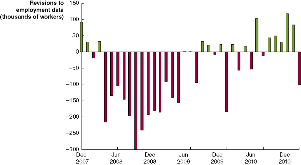
In Macroeconomics, Chapter 9, Section 9.1 (Economics, Chapter 19, Section 19.1), we give an example of substantial revisions in the employment data. Figure 9.5 (reproduced below) shows that the declines in employment during the 2007–2009 recession were initially greatly underestimated. For example, the BLS initially reported that employment declined by 159,000 during September 2008. But after additional data became available, the BLS revised its estimate to a much larger decline of 460,000.

Similarly, in Macroeconomics, Chapter 15, Section 15,3, in the Apply the Concept “Trying to Hit a Moving Target: Making Policy with ‘Real-Time Data’,” we show the BEA’s estimates of the change in real GDP during the first quarter of 2008 have been revised substantially over time. The BEA’s advance estimate of the change in real GDP during the first quarter of 2008 was an increase of 0.6 percent at an annual rate. But that estimate of real GDP growth has been revised a number of times over the years, mostly downward. Currently, BEA data indicate that real GDP actually declined by 1.6 percent at an annual rate during the first quarter of 2008. This swing of more than 2 percentage points from the advance estimate is a large difference, which changes the picture of what happened during the first quarter of 2008 from one of an economy experiencing slow growth to one of an economy suffering a sharp downturn as it fell into the worst recession since the Great Depression of the 1930s.

The changes to the estimates of both employment and real GDP during the beginning of the 2007–2009 recession are not surprising. The initial estimates of employment and real GDP rely on incomplete data. The estimates are revised as additional data are collected by government agencies. During the beginning of a recession, these additional data are likely to show lower levels of employment and output than were indicated by the initial estimates. If the U.S. economy is in a recession in the second quarter of 2022, we can expect that the BLS and BEA will revise their initial estimates of employment and real GDP downward, which—depending on the relative magnitudes of the revisions to the two series—may resolve the paradox of rising employment and falling output. 

Or it’s possible that the U.S. economy is not in a recession. In that case, the employment data may be correct in showing an increase in the number of people working, and the real GDP data may be revised upward to show that output has actually been expanding during the first six months of 2022. Economists and policymakers will have to wait to see which of these alternatives turns out to be the case.

More on Hidden Inflation

This yogurt remained the same price although the container shrank from 5.3 ounces to 4.5 ounces.

Each month, hundreds of employees of the Bureau of Labor Statistics (BLS) gather data on prices of goods and services from stores in 87 cities and from websites. The BLS constructs the consumer price index (CPI) by giving each price a weight equal to the fraction of a typical family’s budget spent on that good or service. (CPI is discussed in Macroeconomics, Chapter 9, Section 9.4 and in Economics, Chapter 19, Section 19.4.) Ideally, the BLS tracks prices of the same product over time. But sometimes a particular brand and style of shirt, for example, is discontinued. In that case, the BLS will instead use the price of a shirt that is a very close substitute.

A more difficult problem arises when the price of a good increases at the same time that the quality of the good improves. For instance, a new model iPhone may have both a higher price and a better battery than the model it replaces, so the higher price partly reflects the improvement in the quality of the phone. The BLS has long been aware of this problem and has developed statistical techniques that attempt to identify which part of the price increases are due to increases in quality. Economists differ in their views on how successfully the BLS has dealt with this quality bias to the measured inflation rate. Because of this bias in constructing the CPI, it’s possible that the published values of inflation may overstate the actual annual rate of inflation by 0.5 percentage point. For instance, the BLS might report an inflation rate of 3.5 percent when the actual inflation rate—if the BLS could determine it—was 4.0 percent.
As the inflation rate increased beginning in the spring of 2021, a number of observers pointed to hidden inflation that was occurring. There were two main types of hidden inflation:

  1. The quality of some services was declining
  2. Some packaged goods contained smaller quantities at the same price

Here’s one example of the deteriorating quality of some services. Because during 2021 and 2022 many restaurants were having difficulty hiring servers, it was often taking longer for customers to have their orders taken and to have their food brought to the table. Because restaurants were also having difficulty hiring enough cooks, they also limited the items available on their menus. In other words, the service these restaurants were offering was not as good as it had been prior to the pandemic. So even if the restaurants kept their prices unchanged, their customers were paying the same price, but receiving less.
Alan Cole, a former senior economist with the Congressional Joint Economic Committee, discussed these other examples on his blog: “hotels clean rooms less frequently on multi-night stays, shipping delays are longer, and phone hold times at airlines are worse.” In a column in the New York Times, economics writer Neil Irwin made similar points: “Complaints have been frequent about the cleanliness of [restaurant] tables, floors and bathrooms.” And: “People trying to buy appliances and other retail goods are waiting longer.”

A column in the Wall Street Journal on business travel by Scott McCartney was headlined “The Incredible Disappearing Hotel Breakfast.” McCartney noted that many hotels continue to advertise free hot breakfasts on their websites and apps but have stopped providing them. He also noted that hotels “have suffered from labor shortages that have made it difficult to supply services such as daily housekeeping or loyalty-group lounges,” in addition to hot breakfasts.
In all of these cases, the actual prices of the services had increased more than had the listed prices because the deterioration in quality meant that people were receiving less for their money.


In addition to deterioration in the quality of services, hidden inflation during this period also took the form of consumers buying some packaged goods in which the quantities had been reduced, although the price was unchanged. For example, in June 2022, an article by the Associated Press noted that:


• “A small box of Kleenex now has 60 tissues; a few months ago, it had 65.”
• “Chobani Flips yogurts have shrunk from 5.3 ounces to 4.5 ounces.”
• “Earth’s Best Organic Sunny Days Snack Bars went from eight bars per box to seven, but the price listed at multiple stores remains $3.69.”


An article in the Wall Street Journal observed that: “Shrinkflation, as economists call it, tends to be easier for companies to pass on to consumers. Despite labels that show price by weight, research shows that most customers look at only the overall price.”


The BLS does try to adjust the measurement of the CPI for shrinkflation, which it can do because the BLS keeps careful track of the quantities included in the packaged goods that are included in its survey.


But the BLS makes no attempt to adjust the CPI for the deterioration in the quality of services because doing so would be very difficult. As Irwin observes: “Customer service preferences—particularly how much good service is worth—varies highly among individuals and is hard to quantify. How much extra would you pay for a fast-food hamburger from a restaurant that cleans its restroom more frequently than the place across the street?” And an economist at the BLS noted that, “We do not capture the decrease in service quality associated with cleaning a [hotel] room every two days rather than one.”


As we noted earlier, most economists believe that the failure of the BLS to fully account for improvements in the quality of goods results in changes in the CPI overstating the true inflation rate. This bias may have been more than offset during 2021–2022 by deterioration in the quality of services resulting in the CPI understating the true inflation rate. As the dislocations caused by the pandemic gradually resolve themselves, it seems likely that the deterioration in services will be reversed. But it’s possible that the deterioration in the provision of some services may persist. Fortunately, unless the deterioration increases over time, it would not continue to distort the measurement of the inflation rate because the same lower level of service would be included in every period’s prices.


Sources: Dee-Ann Durbin, “No, You’re Not Imagining It—Package Sizes Are Shrinking,” apnews.com, June 8, 2022; Annie Gasparro and Gabriel T. Rubin, “The Hidden Ways Companies Raise Prices,” Wall Street Journal, February 12, 2022; Alan Cole, “How I Reluctantly Became an Inflation Crank,” fullstackeconomics.com, September 8, 2021; Scott McCartney, “The Incredible Disappearing Hotel Breakfast—and Other Amenities Travelers Miss,” Wall Street Journal, October 20, 2021; and Neil Irwin, “There Is Shadow Inflation Taking Place All Around Us,” New York Times, October 14, 2021.

Was the High Inflation of 2021–2022 Due to Shifts in Aggregate Demand or Shifts in Aggregate Supply?

Man surprised by inflation in food prices.

To answer the question in the title:  Negative supply shocks—shifts to the left in the short-run aggregate supply (SRSAS) curve—and positive demand shocks—shifts to the right in the aggregate demand (AD) curve—both contributed to the acceleration in inflation that began in the spring of 2021. But were the aggregate supply shifts, such as the semiconductor shortage that reduced the supply of new automobiles, more or less important than the aggregate demand shifts, such as the expansionary monetary and fiscal policies?

Adam Hale Shapiro of the Federal Reserve Bank of San Francisco used a basic piece of microeconomic analysis to estimate the contribution of shifts in aggregate supply and shifts in aggregate demand to inflation during this period. He looked at the prices of the more than 100 categories of goods and services in the personal consumption expenditures(PCEprice index. The PCE price index is a measure of the price level similar to the GDP deflator, except it includes only the prices of goods and services from the consumption category of GDP. Changes in the PCE price index are the Federal Reserve’s preferred measure of the inflation rate because that index includes the prices of more goods and services than are included in the consumer price index (CPI).

Shapiro explains how he used microeconomic reasoning to determine whether prices in one of the more than 100 categories of goods and services were increasing because of shifts in supply or because of shifts in demand:

“Shifts in demand move both prices and quantities in the same direction along the upward-sloping supply curve, meaning prices rise as demand increases. Shifts in supply move prices and quantities in opposite directions along the downward-sloping demand curve, meaning prices rise when supplies decline.”

 For example, the figure on the left shows the effect on the market for toys of an increase in the demand for toys. (We discuss how shifts in demand and supply curves in a market affect equilibrium price and quantity in Chapter 3, Section 3.4 of Economics, Macroeconomics, and Microeconomics.) The demand curve for toys shifts to the right from D1 to D2, the equilibrium price increases from P1 to P2, and the equilibrium quantity increases from Q1 to Q2. The figure on the right shows the effect on the market for toys if the price increase results from a decrease in the supply of toys rather than from an increase in demand. The supply curve shifts to the left from S1 to S2, the equilibrium price increases from P1 to P2, and the equilibrium quantity decreases from Q1 to Q2

Shapiro used statistical methods to determine the part of a change in price or quantity that was unexpected. He took this approach in order to focus on short-run changes in these markets caused by shifts in demand and supply rather than long-run changes resulting from “factors such as technological improvements, cost-of-living adjustments to wages, or demographic changes like population aging.” In some cases, the quantity or the price in a market were very close to their expected values, so Shapiro labeled the cause of a price increase in this market as “ambiguous.”

Shapiro notes that: “Categories that experience frequent supply-driven price changes include food and household products such as dishes, linens, and household paper items. Categories that experience frequent demand-driven price changes include motor vehicle-related products, used cars, and electricity.”

The following figure shows Shapiro’s results for the period from January 2020 through April 2022. The height of each column gives the inflation rate in the month measured as the percentage change in the PCE price index from the same month in the previous year. For example, in March 2022, the inflation rate was 6.6 percent. The height of the yellow segment is the part of inflation in that month attributable to increases in demand, the height of the green segment is the part of the inflation in that month that is attributable to decreases in supply, and the height of the green segment is the part of the inflation that Shapiro can’t assign to either demand or supply. In March 2022, increased in demand accounted for 2.2 percentage points of the total 6.6 percentage point increase in inflation. Decreases in supply accounted for 3.3 percentage points, and the remaining 1.2 percentage points had an ambiguous cause. 

We can conclude that, measured this way, the increase in inflation from the spring of 2021 through the spring of 2022 was due more to negative supply shocks than to positive demand shocks.

Source: Adam Hale Shapiro, “How Much Do Supply and Demand Drive Inflation?” Federal Reserve Bank of San Francisco Economic Letter, 22-15, June 21, 2022.

Are the Fed’s Forecasts of Inflation and Unemployment Inconsistent?

The Federal Reserve building in Washington, DC. Photo from the Wall Street Journal.

Four times per year, the members of the Federal Reserve’s Federal Open Market Committee (FOMC) publish their projections, or forecasts, of the values of the inflation rate, the unemployment, and changes in real gross domestic product (GDP) for the current year, each of the following two years, and for the “longer run.”  The following table, released following the FOMC meeting held on March 15 and 16, 2022, shows the forecasts the members made at that time.

  Median Forecast Meidan Forecast Median Forecast 
 202220232024Longer runActual values, March 2022
Change in real GDP2.8%2.2%2.2%1.8%3.5%
Unemployment rate3.5%3.5%3.6%4.0%3.6%
PCE inflation4.3%2.7%2.3%2.0%6.6%
Core PCE inflation4.1%2.6%2.3%No forecast5.2%

Recall that PCE refers to the consumption expenditures price index, which includes the prices of goods and services that are in the consumption category of GDP. Fed policymakers prefer using the PCE to measure inflation rather than the consumer price index (CPI) because the PCE includes the prices of more goods and services. The Fed uses the PCE to measure whether it is hitting its target inflation rate of 2 percent. The core PCE index leaves out the prices of food and energy products, including gasoline. The prices of food and energy products tend to fluctuate for reasons that do not affect the overall long-run inflation rate. So Fed policymakers believe that core PCE gives a better measure of the underlying inflation rate. (We discuss the PCE and the CPI in the Apply the Concept “Should the Fed Worry about the Prices of Food and Gasoline?” in Macroeconomics, Chapter 15, Section 15.5 (Economics, Chapter 25, Section 25.5)).

The values in the table are the median forecasts of the FOMC members, meaning that the forecasts of half the members were higher and half were lower.  The members do not make a longer run forecast for core PCE.  The final column shows the actual values of each variable in March 2022. The values in that column represent the percentage in each variable from the corresponding month (or quarter in the case of real GDP) in the previous year.  Links to the FOMC’s economic projections can be found on this page of the Federal Reserve’s web site.

At its March 2022 meeting, the FOMC began increasing its target for the federal funds rate with the expectation that a less expansionary monetary policy would slow the high rates of inflation the U.S. economy was experiencing. Note that in that month, inflation measured by the PCE was running far above the Fed’s target inflation rate of 2 percent. 

In raising its target for the federal funds rate and by also allowing its holdings of U.S. Treasury securities and mortgage-backed securities to decline, Fed Chair Jerome Powell and the other members of the FOMC were attempting to achieve a soft landing for the economy. A soft landing occurs when the FOMC is able to reduce the inflation rate without causing the economy to experience a recession. The forecast values in the table are consistent with a soft landing because they show inflation declining towards the Fed’s target rate of 2 percent while the unemployment rate remains below 4 percent—historically, a very low unemployment rate—and the growth rate of real GDP remains positive. By forecasting that real GDP would continue growing while the unemployment rate would remain below 4 percent, the FOMC was forecasting that no recession would occur.

Some economists see an inconsistency in the FOMC’s forecasts of unemployment and inflation as shown in the table. They argued that to bring down the inflation rate as rapidly as the forecasts indicated, the FOMC would have to cause a significant decline in aggregate demand. But if aggregate demand declined significantly, real GDP would either decline or grow very slowly, resulting in the unemployment rising above 4 percent, possibly well above that rate.  For instance, writing in the Economist magazine, Jón Steinsson of the University of California, Berkeley, noted that the FOMC’s “combination of forecasts [of inflation and unemployment] has been dubbed the ‘immaculate disinflation’ because inflation is seen as falling rapidly despite a very tight labor market and a [federal funds] rate that is for the most part negative in real terms (i.e., adjusted for inflation).”

Similarly, writing in the Washington Post, Harvard economist and former Treasury secretary Lawrence Summers noted that “over the past 75 years, every time inflation has exceeded 4 percent and unemployment has been below 5 percent, the U.S. economy has gone into recession within two years.”

In an interview in the Financial Times, Olivier Blanchard, senior fellow at the Peterson Institute for International Economics and former chief economist at the International Monetary Fund, agreed. In their forecasts, the FOMC “had unemployment staying at 3.5 percent throughout the next two years, and they also had inflation coming down nicely to two point something. That just will not happen. …. [E]ither we’ll have a lot more inflation if unemployment remains at 3.5 per cent, or we will have higher unemployment for a while if we are actually to inflation down to two point something.”

While all three of these economists believed that unemployment would have to increase if inflation was to be brought down close to the Fed’s 2 percent target, none were certain that a recession would occur.

What might explain the apparent inconsistency in the FOMC’s forecasts of inflation and unemployment? Here are three possibilities:

  1. Fed policymakers are relatively optimistic that the factors causing the surge in inflation—including the economic dislocations due to the Covid-19 pandemic and the Russian invasion of Ukraine and the surge in federal spending in early 2021—are likely to resolve themselves without the unemployment rate having to increase significantly. As Steinsson puts it in discussing this possibility (which he believes to be unlikely) “it is entirely possible that inflation will simply return to target as the disturbances associated with Covid-19 and the war in Ukraine dissipate.”
  2. Fed Chair Powell and other members of the FOMC were convinced that business managers, workers, and investors still expected that the inflation rate would return to 2 percent in the long run. As a result, none of these groups were taking actions that might lead to a wage-price spiral. (We discussed the possibility of a wage-price spiral in earlier blog post.) For instance, at a press conference following the FOMC meeting held on May 3 and 4, 2022, Powell argued that, “And, in fact, inflation expectations [at longer time horizons] come down fairly sharply. Longer-term inflation expectations have been reasonably stable but have moved up to—but only to levels where they were in 2014, by some measures.” If Powell’s assessment was correct that expectations of future inflation remained at about 2 percent, the probability of a soft landing was increased.
  3. We should mention the possibility that at least some members of the FOMC may have expected that the unemployment rate would increase above 4 percent—possibly well above 4 percent—and that the U.S. economy was likely to enter a recession during the coming months. They may, however, have been unwilling to include this expectation in their published forecasts. If members of the FOMC state that a recession is likely, businesses and households may reduce their spending, which by itself could cause a recession to begin. 

Sources: Martin Wolf, “Olivier Blanchard: There’s a for Markets to Focus on the Present and Extrapolate It Forever,” ft.com, May 26, 2022; Lawrence Summers, “My Inflation Warnings Have Spurred Questions. Here Are My Answers,” Washington Post, April 5, 2022; Jón Steinsson, “Jón Steinsson Believes That a Painless Disinflation Is No Longer Plausible,” economist.com, May 13, 2022; Federal Open Market Committee, “Summary of Economic Projections,” federalreserve.gov, March 16, 2022; and Federal Open Market Committee, “Transcript of Chair Powell’s Press Conference May 4, 2022,” federalreserve.gov, May 4, 2022. 

Does Majoring in Economics Increase Your Income?

Image by Andrea D’Aquino in the Wall Street Journal.

Studying economics provides students in any major with useful tools for understanding business decision making and for evaluating government policies. As we discuss in Chapter 1, Section 1.5 of Microeconomics, Macroeconomics, and Economics, majoring in economics can lead to a career in business, government, or at nonprofit organizations. Many students considering majoring in economics are interested in how the incomes of economics majors compare with the incomes of students who pursue other majors.

            The Federal Reserve Bank of New York maintains a web page that uses data collected by the U.S. Census to show the incomes of people with different college majors. The following table shows for economics majors and for all majors the median annual wage received by people early in their careers and in the middle of their careers. The median is a measure of the average calculated as the annual wage at which half of people in the group have a higher annual wage and half have a lower annual wage. “Early career” refers to people aged 22 to 27, and “mid-career” refers to people aged 35 to 45.  The data are for people with a bachelor’s degree only, so people with a masters or doctoral degree are not included.  

 Median Wage Early CareerMedian Wage Mid-Career
Economics majors$55,000$93,000
All majors$42,000$70,000

The table shows that early in their careers, on average, economics majors earn an annual wage about 31 percent higher than annual wage earned by all majors. At mid-career, in percentage terms, the gap increases slightly to 33 percent.

            How should we interpret these data? In Chapter 1, Section 1.3, in discussing how to evaluate economic models, we made the important distinction between correlation and causality. Just because two things are correlated, or happen at the same time, doesn’t mean that one caused the other. In this case, are the higher than average incomes of economics majors caused by majoring in economics or is majoring in economics correlated with higher incomes, but not actually causing the higher incomes. It might be true, for instance, that on average economics majors have certain characteristics—such as being more intelligent or harder workers—than are students who choose other majors. Because being intelligent and working hard can lead to successful careers, students majoring in economics might have earned higher incomes on average even if they had chosen a different major.

(Here’s a  more advanced point about identifying causal relationships in data: The problem with determining causality described in the previous paragraph is called selection bias. Students aren’t randomly assigned majors; they choose, or self-select, them. If students with characteristics that make it more likely that they will earn high incomes are also more likely to choose to major in economics, then the higher incomes earned by economics majors weren’t caused by (or weren’t entirely caused by) majoring in economics.)

            Economists Zachary Bleemer of the University of California, Berkeley and Aashish Mehta of the University of California, Santa Barbara have found a way to evaluate whether majoring in economics causes students to earn higher incomes. The authors gathered data on all the students admitted to the University of California, Santa Cruz (UCSC) between 2008 and 2012 and on their incomes in 2017 and 2018. To major in economics, students at UCSC needed a grade point average (GPA) of 2.8 or higher in the two principles of economics courses. The authors compared the choices of majors and the average early career earnings of students who just met or just failed to meet the 2.8 GPA threshold for majoring in economics. The authors use advanced statistical analysis to reach the conclusion that: “Comparing the major choices and average wages of above-and-below-threshold students shows that majoring in economics caused a $22,000 (46 percent) increase in annual early-career wages of barely above-threshold students.” 

            The authors attribute half of the higher wages earned by economics majors to their being more likely to pursue careers in finance, insurance, real estate, and accounting, which tend to pay above average wages.  The authors note that their findings from this study “imply that students’ major choices could have financial implications roughly as large as their decision to enroll in college ….”

Sources: Federal Reserve Bank of New York, The Labor Market for Recent College Graduates, https://www.newyorkfed.org/research/college-labor-market/index.html; and Zachary Bleemer and Aashish Meta, “Will Studying Economics Make You Rich? A Regression Discontinuity Analysis of the Returns to College Major,” American Economic Journal: Applied Economics, Vol. 14, No. 2, April 2022, pp. 1-22.

Harvard Professor Edward Glaeser on the Importance of Working on Site

Recently Tunku Varadarajan of the Wall Street Journal interviewed Edward Glaeser on whether the increases in working remotely due to the pandemic are likely to persist.

Glaeser notes that compared with the period before the pandemic, office attendance is still down 19% nationwide. In some large cities, it’s down considerably more, including being down more than 50% in San Francisco and 32% in New York and Boston.

Glaeser believes that a decline in working on site can be a particular problem for young workers:

“Cities—and face-to-face contact at work—have ‘this essential learning component that is valuable and crucial for workers who are young,’ [Glaeser] says. The acquisition of experience and improvement in productivity, ‘month by month, year by year,’ ensures that individual earnings are higher in cities than elsewhere.”

According to Glaeser, people who work remotely face a 50% reduction in the probably of being promoted.

Glaeser is not a fan of remote teaching:

“Delivering a lecture to 100 students on Zoom, he says, is ‘just a bad movie, a really bad movie. None of the magic that comes from live lecturing and live interaction with students is there when you’re doing it via Zoom.'”

There is much more in the article, which is well worth reading. It can be found here (a subscription may be required).

A Day in the Life of a Price Checker for the Bureau of Labor Statistics

Emily Mascitis checks prices at an auto-repair shop in Philadelphia. (Photo from the Wall Street Journal.)

As we discuss in Macroeconomics, Chapter 9, Section 9.4, (Economics, Chapter 19, Section 19.4) in calculating the consumer price index (CPI) each month, the Bureau of Labor Statistics sends hundreds of employees to gather price data from stores and offices. A reporter for the Wall Street Journal followed a price checker as she visited an auto-repair shop, a grocery store, and other businesses.

The article provides an excellent discussion of the care with which prices are collected, particularly with respect to making sure that the prices are for the same good or service each month. For instance, while in a grocery, the price checker almost made the mistake of recording the price of a can of low sodium chicken noodle soup, rather than the price of regular chicken noodle soup as in previous months.

At one point, the price checker noted that the price of clementines had been increasing rapidly and remarked that when buying fruit for her own family “We need to pick a less expensive fruit.” Switching from buying a fruit, in this case clementines, with a price that is increasing rapidly to a fruit with a price that is increasing more slowly, say regular oranges, is an example of the substitution bias. That’s one of the four biases discussed in Section 9.4 that can cause the measured increase in the CPI to overstate the true rate of inflation.

The article can be found here. (A subscription may be required.)

Source: Rachel Wolfe, “How the Inflation Rate Is Measured: 477 Government Workers at Grocery Stores,” Wall Street Journal, May 10, 2022.

Interest Rates, the Yen, the Dollar, and the International Financial System 

Photo from the Wall Street Journal.

From early March to early May 2022, the Japanese yen persistently lost value versus the U.S. dollar. Between March 1 and May 9, the yen declined by 14% against the dollar, which is a substantial loss in value during such a short time period.  What explains the decline in the exchange rate between the yen and the dollar during that time? In Macroeconomics, Chapter 18, Section 18.2 (Economics, Chapter 28, Section 28.2), we saw that the exchange rate between most pairs of currencies fluctuates in response to these factors:

  • The foreign demand for U.S. goods
  • U.S. interest rates relative to foreign interest rates
  • Foreign demand for making direct investments or portfolio investments in the United States
  • The U.S. demand for foreign goods
  • Foreign interest rates relative to U.S interest rates
  • U.S. demand for making direct investments or portfolio investments in other countries

The following figure shows movements in the exchange rate between the yen and the U.S. dollar since 2010.  During different periods, the factor that is most important in explaining fluctuations in an exchange rate varies.  (Important note: The figure follows the convention of expressing the exchange between the yen and dollar in terms of yen per dollar. Therefore, in the figure, an increase in the exchange rate corresponds to a decrease in the value of the yen versus the dollar because it takes more yen to buy one dollar.)

From early March to early May 2022, the decline in value of the yen versus the dollar was mainly the result of U.S. interest rates increasing relative to Japanese interest rates. As the inflation rate increased rapidly in the spring of 2022, both short-term and long-term interest rates in the United States increased, partly in response to policy actions taken by the Federal Reserve. The Federal Reserve was attempting to increase interest rates in order to raise borrowing costs for households and firms, thereby slowing spending and inflation.  Japan was experiencing much lower rates of inflation—well below the Bank of Japan’s 2% annual inflation target—so the BOJ was reluctant to increase interest rates. As a consequence, the gap between the interest rate on 10-year U.S. Treasury notes and the interest rate on 10-year Japanese government bonds had risen to 2.9 percentage points.

Higher U.S. interest rates caused a shift to the right in the demand for dollars in exchange for yen as foreign investors exchanged their yen for dollars in order to buy U.S. Treasury securities and other U.S. financial assets.  As we show in Chapter 18, Figure 18.13, an increase in the demand for dollars (holding all other factors constant) increases the equilibrium exchange rate between the yen and the dollar.  

What effect does a stronger dollar and a weaker yen have on the two countries’ economies?  A weaker yen means that the yen price of imports from the United States will be higher. The higher prices will increase the Japanese inflation rate, but with inflation being low in in the spring of 2022, Japanese policymakers weren’t concerned by this effect. And because the value of U.S. imports is small relative to the size of the Japanese economy, the effect on the inflation rate wouldn’t be large in any case. The dollar price of Japanese exports to the United States will be lower, which should help Japanese firms exporting to the United States.

The effect on the U.S. economy will be the mirror image of the effect on the Japanese economy. The dollar price of Japanese imports being lower will help reduce the U.S. inflation rate, but not to a great extent because the value of Japanese imports is small relative to the size of the U.S. economy. The yen price of U.S. exports to Japan will be higher, which will be bad news for U.S. firms exporting to Japan.

Finally, many banks, other financial firms, and non-financial firms borrow money in dollars. They do so because over time the advantages of borrowing dollars has increased, even for foreign firms that receive most of their revenue in their domestic currency rather than dollars. In particular, the value of the dollar is relatively stable compared with the value of many other currencies. In addition, the Federal Reserve has made available short-term dollar loans to foreign central banks that allow those banks to provide short-term loans to local firms that are having temporary difficulty making dollar payments on their loans. By late 2021, the total amount of dollar loans made outside of the United States had risen to more than $13 trillion. In the spring of 2022, the value of the dollar was rising not just against the Japanese yen but also against many other currencies. The increase was bad news for foreign firms borrowing in U.S. dollars because it would take more of their domestic currency to buy the dollars necessary to make their loans payments. A large and prolonged increase in the value of the U.S. dollar could possibly upset the stability of the international financial system. 

Sources:  Yuko Takeo and Komaki Ito, “Japan’s Stepped-Up Warnings Fail to Stem Yen’s Slide Past 128,” bloomberg.com, April 19, 2022; Jacky Wong, “Japan Gets a Taste of the Wrong Type of Inflation,” Wall Street Journal, April 1, 2022; Megumi Fujikawa, “Yen Hits Lowest Level Since 2015, and Japan, U.S. Are OK With That,” Wall Street Journal, March 28, 2022; Bank for International Settlements, “BIS International Banking Statistics and Global Liquidity Indicators at End-September 2021,” January 28, 2022; and Federal Reserve Bank of St. Louis.

Are We at the Start of a Recession?

On Thursday morning, April 28, the Bureau of Economic Analysis (BEA) released its “advance” estimate for the change in real GDP during the first quarter of 2022. As shown in the first line of the following table, somewhat surprisingly, the estimate showed that real GDP had declined by 1.4 percent during the first quarter. The Federal Reserve Bank of Atlanta’s “GDP Now” forecast had indicated that real GDP would increase by 0.4 percent in the first quarter. Earlier in April, the Wall Street Journal’s panel of academic, business, and financial economists had forecast an increase of 1.2 percent. (A subscription may be required to access the forecast data from the Wall Street Journal’s panel.)

Do the data on real GDP from the first quarter of 2022 mean that U.S. economy may already be in recession? Not necessarily, for several reasons:

First, as we note in the Apply the Concept, “Trying to Hit a Moving Target: Making Policy with ‘Real-Time’ Data,” in Macroeconomics, Chapter 15, Section 15.3 (Economics, Chapter 25, Section 25.3): “The GDP data the BEA provides are frequently revised, and the revisions can be large enough that the actual state of the economy can be different for what it at first appears to be.”

Second, even though business writers often define a recession as being at least two consecutive quarters of declining real GDP, the National Bureau of Economic Research has a broader definition: “A recession is a significant decline in activity across the economy, lasting more than a few months, visible in industrial production, employment, real income, and wholesale-retail trade.” Particularly given the volatile movements in real GDP during and after the pandemic, it’s possible that even if real GDP declines during the second quarter of 2022, the NBER might not decide to label the period as being a recession.

Third, and most importantly, there are indications in the underlying data that the U.S. economy performed better during the first quarter of 2022 than the estimate of declining real GDP would indicate. In a blog post in January discussing the BEA’s advance estimate of real GDP during the fourth quarter of 2021, we noted that the majority of the 6.9 percent increase in real GDP that quarter was attributable to inventory accumulation. The earlier table indicates that the same was true during the first quarter of 2022: 60 percent of the decline in real GDP during the quarter was the result of a 0.84 decline in inventory investment.

We don’t know whether the decline in inventories indicates that firms had trouble meeting demand for goods from current inventories or whether they decided to reverse some of the increases in inventories from the previous quarter. With supply chain disruptions continuing as China grapples with another wave of Covid-19, firms may be having difficulty gauging how easily they can replace goods sold from their current inventories. Note the corresponding point that the decline in sales of domestic product (line 2 in the table) was smaller than the decline in real GDP.

The table below shows changes in the components of real GDP. Note the very large decline exports and in purchases of goods and services by the federal government. (Recall from Macroeconomics, Chapter 16, Section 16.1, the distinction between government purchases of goods and services and total government expenditures, which include transfer payments.) The decline in federal defense spending was particularly large. It seems likely from media reports that the escalation of Russia’s invasion of Ukraine will lead Congress and President Biden to increase defense spending.

Notice also that increases in the non-government components of aggregate demand remained fairly strong: personal consumption expenditures increased 2.7 percent, gross private domestic investment increased 2.3 percent, and imports surged by 17.7 percent. These data indicate that private demand in the U.S. economy remains strong.

So, should we conclude that the economy will shrug off the decline in real GDP during the first quarter and expand during the remainder of the year? Unfortunately, there are still clouds on the horizon. First, there are the difficult to predict effects of continuing supply chain problems and of the war in Ukraine. Second, the Federal Reserve has begun tightening monetary policy. Whether Fed Chair Jerome Powell will be able to bring about a soft landing, slowing inflation significantly while not causing a large jump in unemployment, remains the great unknown of economic policy. Finally, if high inflation rates persist, households and firms may respond in ways that are difficult to predict and, may, in particular decide to reduce their spending from the current strong levels.

In short, the macroeconomic forecast is cloudy!

Source: The BEA’s web site can be found here.

You’ve Decided to Buy Twitter, So Who Are You Going to Call?  Investment Banks, of Course

Elon Musk. (Photo from the Associated Press.)

That’s what Elon Musk did in April 2022.  In early April, Musk purchased about 9% of Twitter’s shares.  On April 25, he became the owner of Twitter by buying the roughly 90% remaining shares for $54.20 per share. The total he paid for these remaining shares came to $44 billion. Following his often unorthodox style, Musk announced his plans in a tweet on Twitter. Where did he get the money to fund such a large purchase? 

According to Forbes magazine, in March 2022, Musk was by far the richest person in the world with total wealth of about $270 billion—nearly $100 billion more than Amazon founder Jeff Bezos, who is the second-richest person.  While it appears that Musk could afford to buy Twitter without having to borrow any money,  Bloomberg estimated that in April 2022 Musk had only $3 billion in cash. Much of his wealth was in Tesla stock or his ownership shares in SpaceX and the Boring Company, both of which are private companies that, therefore, don’t have publicly traded stock. Musk was reluctant to fund all of his offer for Twitter by selling Tesla stock or finding investors willing to buy into SpaceX and Boring.

Musk turned to investment banks to help him raise the necessary funds. Investment banks, such as Goldman Sachs, differ from commercial banks in that they don’t accept deposits, and they rarely lend directly to households. Instead, investment banks have traditionally concentrated on providing advice to firms issuing stocks and bonds or to firms (and billionaires!) who are looking for ways to finance mergers or acquisitions.  A syndicate of investment banks, including Morgan Stanley (which served as Musk’s lead adviser), Bank of America, Barclays, and what an article in the Wall Street Journal described as “nearly every global blue-chip investment bank aside from the two [Goldman Sachs and JP Morgan Chase] advising Twitter,” put together the following financing package. Initially, Musk wanted to raise $46.5 billion in financing—more than in the end he needed. Of that amount, Musk would provide $21 billion and the investment banks would provide loans for the remaining $25.5 billion. As collateral for the loans, Musk pledged $60 billion of his Tesla stock. 

Musk’s financing was a combination of equity—the $21 billion in cash—and debt—the $25.5 billion in loans from investment banks. To fund his equity investment, he was considering selling some of his stock in Tesla but hoped to attract other equity investors who would put up cash in exchange for part ownership of Twitter. According to press reports, Apollo Global Management, a private equity firm was considering becoming an equity investor. (As we saw in Chapter 9, Section 9.2, private equity firms raise equity capital to invest in other firms.)  Musk’s purchase is called a leveraged buyout (LBO) because (1) he relied  on borrowing for a substantial part of his purchase of Twitter and  (2) he intended to take the company private—the company would no longer have publicly traded stock.

Why would Musk want to buy Twitter? He shared the view of some industry analysts that Twitter’s management had failed to take advantage of opportunities to increase the firm’s profit. The actions of Musk and the investment banks were part of the market for corporate control. As we discuss in Microeconomics, Chapter 8, Section 8.1 (Macroeconomics, Chapter 6, Section 6.1), in large corporations there is often a separation of ownership from control. Although the shareholders legally own the firm, the firm’s top management controls the firm’s day-to-day operations. The result can be a principal-agent problem with the management of a large firm failing to act in the best interests of the firm’s shareholders. The existence of a market for corporate control in which outsiders buy stakes in firms that appear to be poorly managed can make firms more efficient by overcoming these moral hazard problems.

             But Musk had another reason for buying Twitter. As he stated in an interview, “Having a public platform that is maximally trusted and broadly inclusive is extremely important to the future of civilization.”  It was unclear whether this and similar statements meant that  after gaining control of Twitter he might take actions that won’t necessarily increase the firm’s profitability. 

            Elon Musk’s purchase of Twitter is a high profile example of the role that investment banks can play in determining control of large corporations. 

Sources: Kurt Wagner, “Elon Musk Lands Deal to Take Twitter Private for $44 Billion,” bloomberg.com, April 25, 2022; Cara Lombardo and Liz Hoffman, “How Elon Musk Won Twitter,” Wall Street Journal, April 25, 2022; Michele F. Davis, “Elon Musk Vets Potential Equity Partners for Twitter Bid,” bloomberg.com, April 21, 2022; Sabrina Escobar, “Elon Musk Isn’t Twitter’s Only Problem. It Faces a Number of Short-Term Headwinds,” barrons.com, April 21, 2022; Cara Lombardo and Liz Hoffman, “Elon Musk Says He Has $46.5 Billion in Funding for Twitter Bid,” Wall Street Journal, April 21, 2022; Andrew Ross Sorkin, Jason Karaian, Vivian Giang, Stephen Gandel, Lauren Hirsch, Ephrat Livni, and Anna Schaverien, “Elon Musk Wants All of Twitter,” New York Times, April 14, 2022; Rob Copeland, Rebecca Elliott, and Cara Lombardo, “Elon Musk Makes $43 Billion Bid for Twitter, Says ‘Civilization’ At Stake,” Wall Street Journal, April 14, 2022; “The World’s Real-Time Billionaires,” forbes.com, April 24, 2022; Musk’s tweet announcing his offer to buy Twitter can be found here.