Photo from Lena Buonanno
When the Bureau of Labor Statistics’ Employment Situation report is released on the first Friday of each month economists and policymakers—notably including the members of the Federal Reserve’s Federal Open Market Committee (FOMC)—focus on the change in total nonfarm payroll employment as recorded in the establishment, or payroll, survey. That number gives what is generally considered to be the best indicator of the current state of the labor market. The most recent report showed a surprisingly strong net increase of 336,000 jobs during September. (The report can be found here.)
According to a survey by the Wall Street Journal, economists had been expecting an net increase in jobs of only 170,000. The larger than expected increase indicated that the economy might be expanding more rapidly than had been thought, raising the possibility that the FOMC might increase its target for the federal funds rate at least once more before the end of the year.
To meet increases in the growth of the U.S. working-age population, the economy needs to increase the total jobs available by approximately 80,000 jobs per month. A net increase of more than four times that amount may be an indication of an overheated job market. As always, one difficulty with drawing that conclusion is determing how many more people might be pulled into the labor market by a strong demand for workers. An increase in labor supply can potentially satisify an increase in labor demand without leading to an acceleration in wage growth and price inflation.
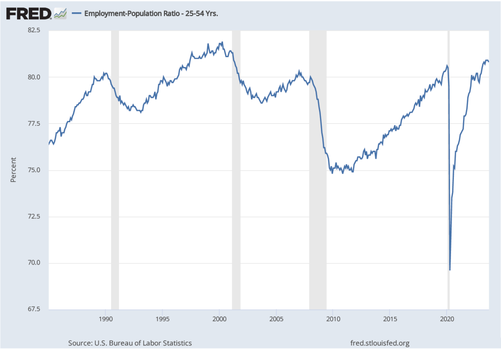
The following figure shows the employment-to-population ratio for workers ages 25 to 54—so-called prime-age workers—for the period since 1985. In September 2023, the ratio was 80.8 perccent, down slightly from 80.9 percent in August, but above the levels reached in early 2020 just before the effects of the Covid–19 pandemic were felt in the United States. The ratio was still below the record high of 81.9 percent reached in April 2000. The population of prime-age workers is about 128 million. So, if the employment-population ratio were to return to its 2000 peak, potentially another 1.3 million prime-age workers might enter the labor market. The likelihood of that happening, however, is difficult to gauge.
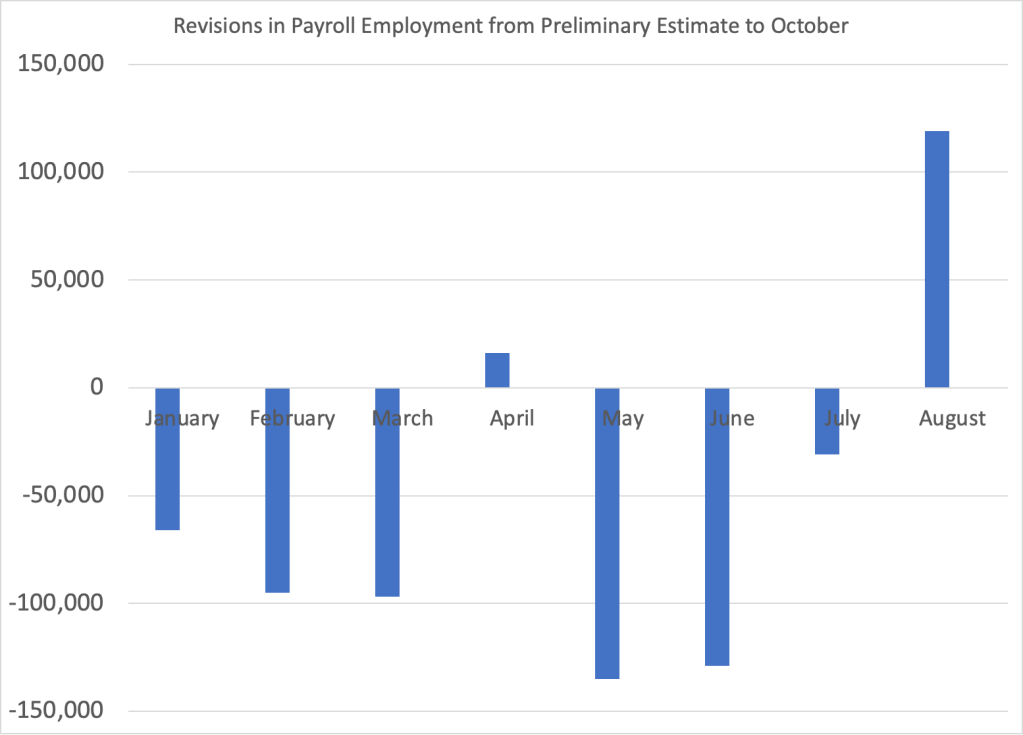
A couple of other points about the September employment report. First, it’s worth keeping in mind that the results from the establishment survey are subject to often substantial revisisons. The figure below shows the revisions the BLS has released as of October to their preliminary estimates for each month of 2023. In three of these eight months the revisions so far have been greater than 100,000 jobs. As we discuss in Macroeconomics, Chapter 9, Section 9.1 (Economics, Chapter 19, Section 19.1 and Essentials of Economics, Chapter 13, Section 13.1), the revisions that the BLS makes to its employment estimates are likely to be particularly large when the economy is about to enter a period of significantly lower or higher growth. So, the large revisions to the preliminary employment estimates in most months of 2023 may indicate that the surprisingly large preliminary estimate of a 336,000 increase in net employment will be revised lower in coming months.
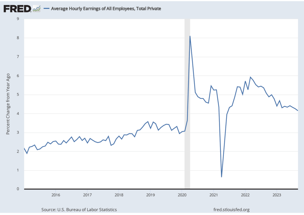
Finally, data in the employment report provides some evidence of a slowing in wage growth, despite the sharp increase in employment. The following figure shows wage inflation as measured by the percentage increase in average hourly earnings (AHE) from the same month in the previous year. The increase in September was 4.2 percent, continuing a generally downward trend since March 2022, although still somewhat above wage inflation during the pre-2020 period.
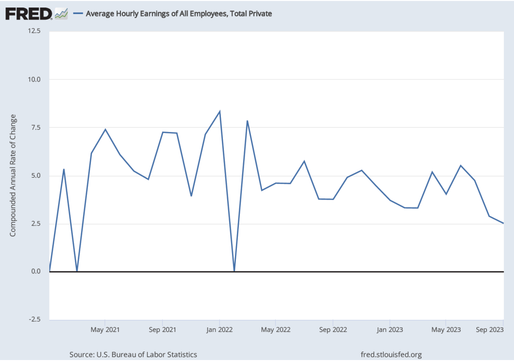
As the following figure shows, September growth in average hourly earnings measured as a compound annual growth rate was 2.5 percent, which—if sustained—would be consistent with a rate of price inflation in the range of the Fed’s 2 percent target. (The figure shows only the months since January 2021 to avoid obscuring the values for recent months by including the very large monthly increases and decrease during 2020.)
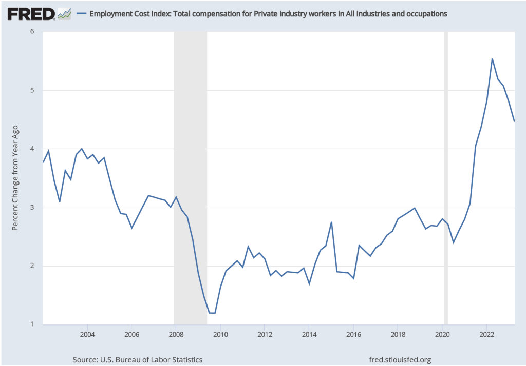
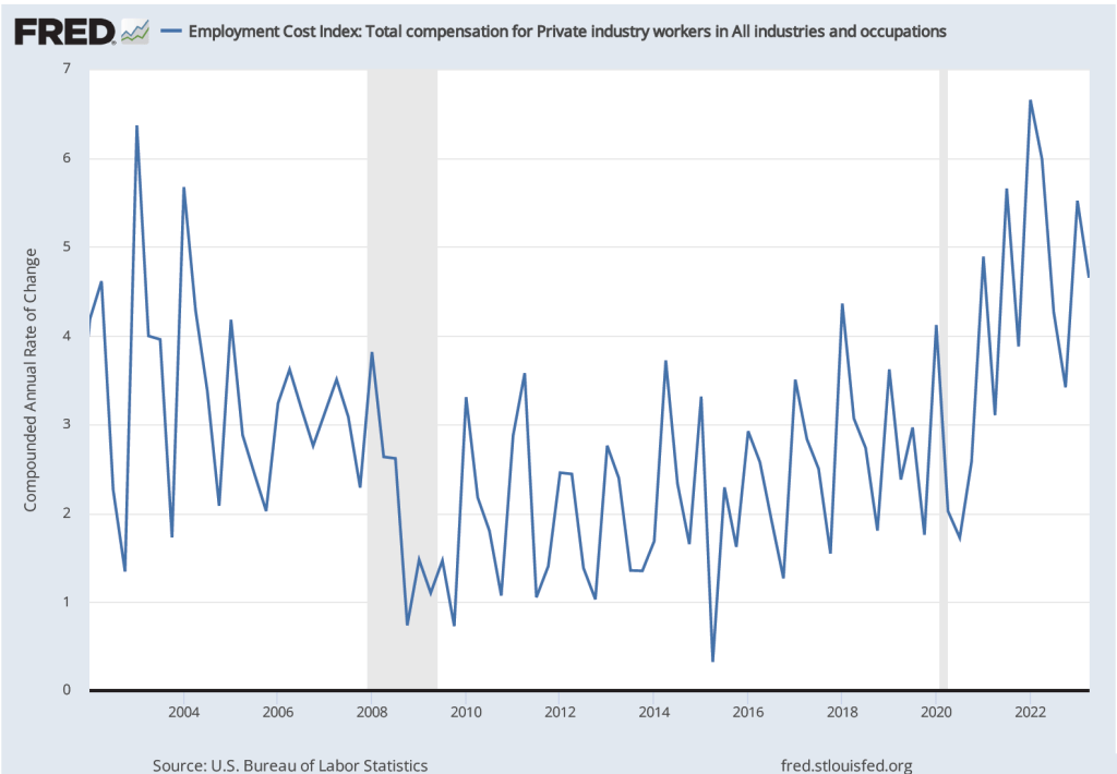
As we note in this blog post, the employment cost index (ECI), published quarterly by the BLS, measures the cost to employers per employee hour worked and can be a better measure than AHE of the labor costs employers face. The first figure shows the percentage change in ECI from the same quarter in the previous year. The second figure shows the compound annual growth rate of the ECI. Both measures show a general downward trend in the growth of labor costs, although the measures are somewhat dated because the most recent values are for the second quarter of 2023.
Ultimately, the key question is one we’ve considered in previous blog posts (most recently here) and podcasts (most recently here): Will the Fed be able to achieve a soft landing by bringing inflation down to its 2 percent target without triggering a recession? The September jobs report can be interpreted as increasing the probability of a soft landing if the slowing in wage growth is emphasized but decreasing the probability if the Fed decides that the strong employment growth is real—that is, the September increase is not likely to be revised sharply lower in coming months—and requires additional increases in the target for the federal funds rate. It’s worth mentioning, of course, that factors over which the Fed has no control, such as a federal government shutdown, rising oil prices, or uncertainty resulting from the attack on Israel by Hamas, will also affect the likelihood of a soft landing.