
Join authors Glenn Hubbard and Tony O’Brien as they discuss the future of small banks in the US financial system in the wake of recent bank failures. With a government that is guaranteeing just about all deposits, what is the role of deposit insurance. Small banks serve a real purpose in our economy and will further government regularly only complicate their mission. Other small business rely on small banks for their intimate knowledge of their market and of their business. However, many may now rely on larger banks that may seem a safer place over the next few years. Our discussion covers these points but you can also check for updates on our blog post that can be found HERE .
Category: Macroeconomics
New York Fed Economists Analyze the Decline in the Labor Force Participation Rate

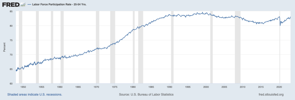
The ability of any economy to produce goods and services depends partly on the number of people working in the economy. The number of people working depends on the size of the population and the fraction of the population that is working. As we discuss in Macroeconomics, Chapter 9, Section 9.1 (Economics, Chapter 19, Section 9.1), the labor force participation rate (LFPR) is the fraction of the working-age population in the labor force. (Technically, the “working-age population” is the civilian, non-institutional population age 16 and older.)
The figure above shows the values of the LFPR from January 1948 through February 2023. The steady increase in the LFPR beginning in the late 1960s and lasting until 2000 was caused by an increase in the number of women working outside of the home and the effects of the baby boom–the increase in birth rates between 1946 and 1964–which led to a decline in the average age of the U.S. population. The LFPR reached a peak of 67.3 percent in early 2000. The gradual decline in the following years reflects the aging of the population as birth rates fell and a small decline in the fraction of prime-age workers–those between ages 25 and 54–in the labor force.
The start of the Covid-19 pandemic in the United States in March 2020 led to an abrupt decline in the LFPR followed by a gradual recovery. In February 2020, the LFPR was 63.3 percent. In February 2023, it was 62.5 percent. The difference means that about 2.1 million fewer people were working in February 2023 than would have been working if the LFPR had regained its February 2020 level.
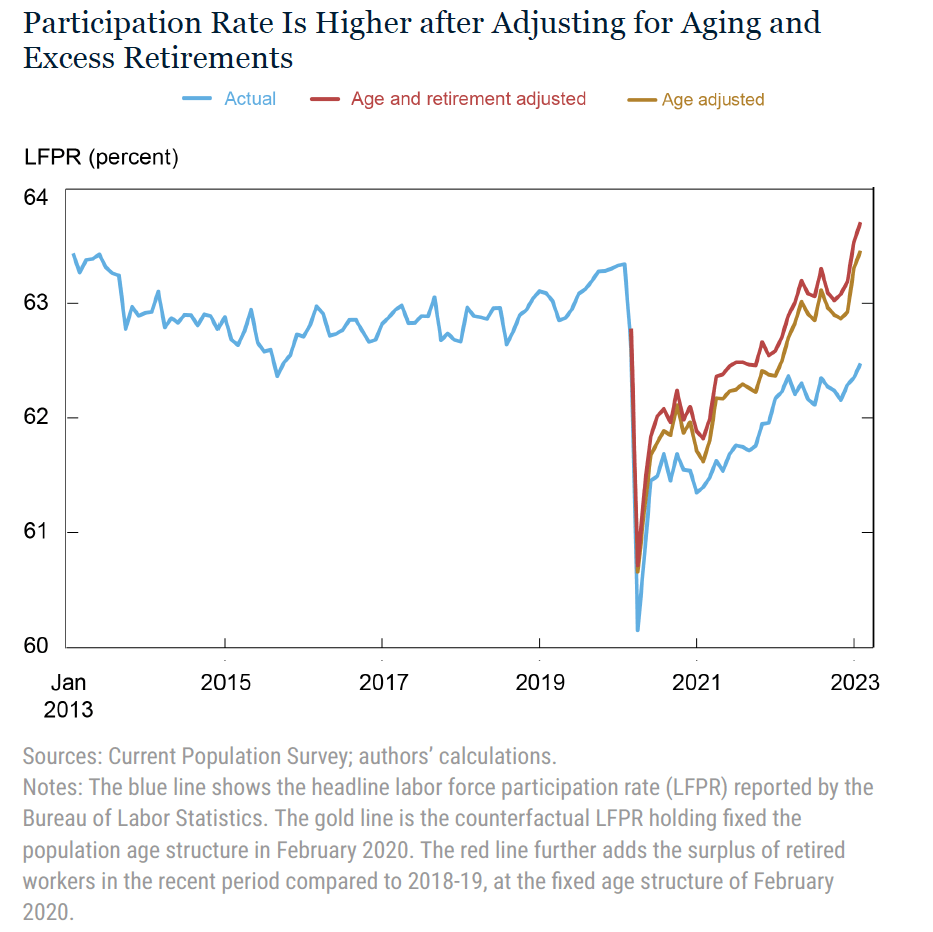
What explains the LFPR not regaining is pre-Covid level? The following figure shows that in February 2023, the LFPR for prime-age workers had reached its February 2020 level. The implication of the figure is that the decline in the LFPR for the whole working-age population is due to a decline in labor force participation by non-prime-age workers.
This conclusion is confirmed by the analys of economists Mary Amiti, Sebastian Heise, Giorgio Topa, and Julia Wu of the Federal Reserve Bank of New York. (Their paper can be found here.) They consider three possible explanations for the decline in the overall LFPR:
- The aging of the U.S. population
- An increase in fraction of people in different age groups who have retired
- An increase in the fraction of the population that is disabled, as result of suffering from “long Covid” or for other reasons
After analyzing the data they find that an increase in retirement rates (explanation 2), particularly for older people, has had only a small effect on LFPR. They find that “Once we adjust for aging, we find that the share of disabled individuals not in the labor force has, in fact, marginally declined.” So explanation 3 is not the key to the decline in the LFPR. They conclude that 1 is the most likely explanation: “Removing the effect of aging can explain the entire participation gap ….” The figure below summarizes their results. The gold line shows that if the United States had the same age structure in February 2023 as it had in February 2020 (that is, if the average age of the working population were lower, with fewer people older than 65), the LFPR would not have declined.
The FDIC Finds a Buyer for Silicon Valley Bank
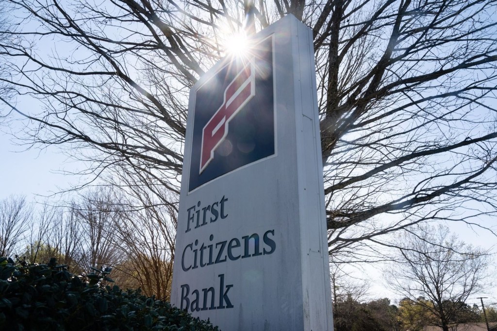
First Citizens Bank, based in based in Raleigh, North Carolina has purchased Silicon Valley Bank. Photo from the Wall Street Journal.
When the Federal Deposit Insurance Corporation (FDIC) took over Silicon Valley Bank (SVB) on March 10, 2023, it kept the bank in operation by setting up a “bridge bank.” The Silicon Valley Bridge Bank kept SVB’s branches running and allowed depositors–including those with deposits above the FDIC’s $250,000 insurance limit–to withdraw funds. The Silicon Valley Bridge Bank borrowed from the Federal Reserve Bank of San Francisco to ensure that it had the funds available to meet deposit withdrawals.
The FDIC prefers to use bridge banks to operate failed banks for as short a time as possible. Typically, the FDIC will seize a bank on a Friday and ideally will have identified another commercial bank willing to purchase the seized bank by the start of business on the following Monday. Finding a bank to buy SVB proved difficult, however, for two reasons:
1. The Biden administration has been skeptical of increasing concentration in the banking industry. That fact may have kept the FDIC from attempting to recruit a large bank to buy SVB, or large banks may have been reluctant to buy SVB because they believed that the Federal Trade Commission or the antitrust division of the U.S. Department of Justice would have blocked the purchase or would have imposed restrictions on how the bank could be operated.
2. Following the Great Financial Crisis of 2008-2009, some banks that purchased failing financial firms found themselves having to deal with loans and securities that had declined in value and with lawsuits from investors in the bank. That history may have caused many banks to be reluctant to buy SVB.
After two attempts to auction SVB failed to attract a buyer, on Sunday, March 26, the FDIC announced that First Citizens Bank, a regional bank based in Raleigh, North Carolina had agreed to purchase SVB. Before the merger, First Citizens was the thirtieth largest bank in the United States, so its purchase of SVB would not significantly increase concentration in retail banking.
Under terms of the purchase, on Monday morning First Citizens began operating SVB’s 17 branches, which now become First Citizens’ branches, assumed responsibility for SVBs deposits, and received $70 billion in SVB’s assets, at a 16.5 percent discount. About $90 billion in SVB’s assets will remain with the FDIC until a buyer for them can be found. The FDIC believes it will have lost about $20 billion from its Deposit Insurance Fund (DIF) as a result of the SVB’s failure. The FDIC will use a special levy on commercial banks to replenish the DIF.
The FDIC’s announcement of First Citizens’ purchase of SVB can be found here.
Why Don’t Financial Markets Believe the Fed?
Fed Chair Jerome Powell holding a news conference following the March 22 meeting of the FOMC. Photo from Reuters via the Wall Street Journal.
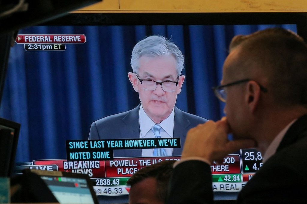
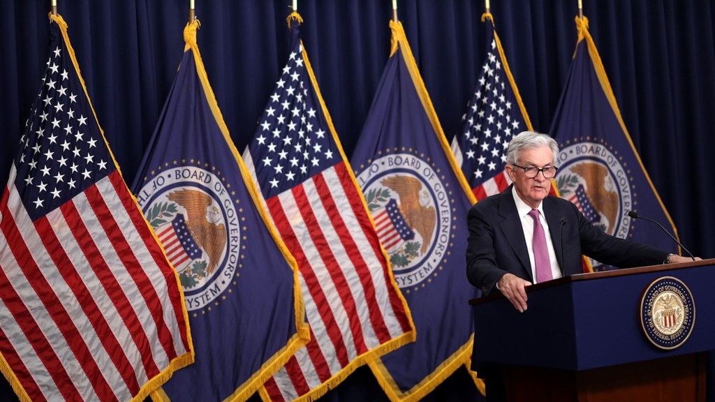
On March 22, the Federal Open Market Committee (FOMC) unanimously voted to raise its target for the federal funds rate by 0.25 percentage point to a range of 4.75 percent to 5.00 percent. The members of the FOMC also made economic projections of the values of certain key economic variables. (We show a table summarizing these projections at the end of this post.) The summary of economic projections includes the following “dot plot” showing each member of the committee’s forecast of the value of the federal funds rate at the end of each of the following years. Each dot represents one member of the committee.
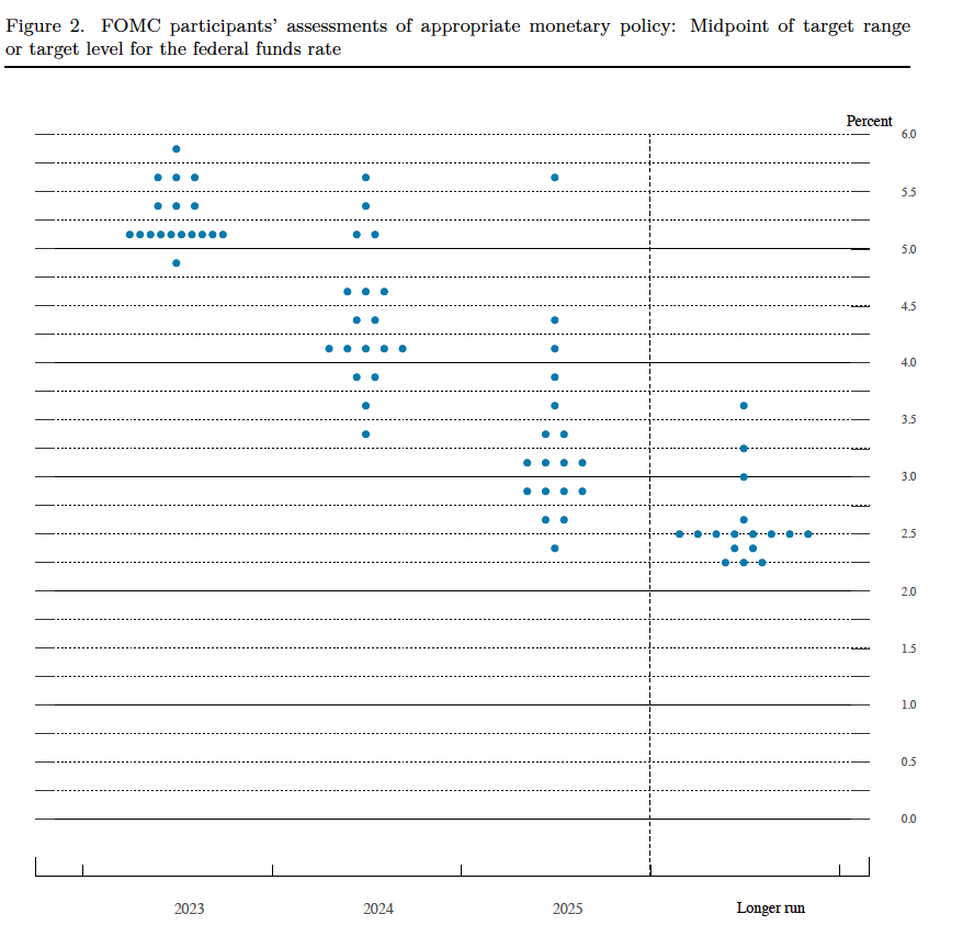
If you focus on the dots above “2023” on the vertical axis, you can see that 17 of the 18 members of the FOMC expect that the federal funds rate will end the year above 5 percent.
In a press conference after the committee meeting, a reporter asked Fed Chair Jerome Powell was asked this question: “Following today’s decision, the [financial] markets have now priced in one more increase in May and then every meeting the rest of this year, they’re pricing in rate cuts.” Powell responded, in part, by saying: “So we published an SEP [Summary of Economic Projections] today, as you will have seen, it shows that basically participants expect relatively slow growth, a gradual rebalancing of supply and demand, and labor market, with inflation moving down gradually. In that most likely case, if that happens, participants don’t see rate cuts this year. They just don’t.” (Emphasis added. The whole transcript of Powell’s press conference can be found here.)
Futures markets allow investors to buy and sell futures contracts on commodities–such as wheat and oil–and on financial assets. Investors can use futures contracts both to hedge against risk–such as a sudden increase in oil prices or in interest rates–and to speculate by, in effect, betting on whether the price of a commodity or financial asset is likely to rise or fall. (We discuss the mechanics of futures markets in Chapter 7, Section 7.3 of Money, Banks, and the Financial System.) The CME Group was formed from several futures markets, including the Chicago Mercantile Exchange, and allows investors to trade federal funds futures contracts. The data that result from trading on the CME indicate what investors in financial markets expect future values of the federal funds rate to be. The following chart shows values after trading of federal funds futures on March 24, 2023.
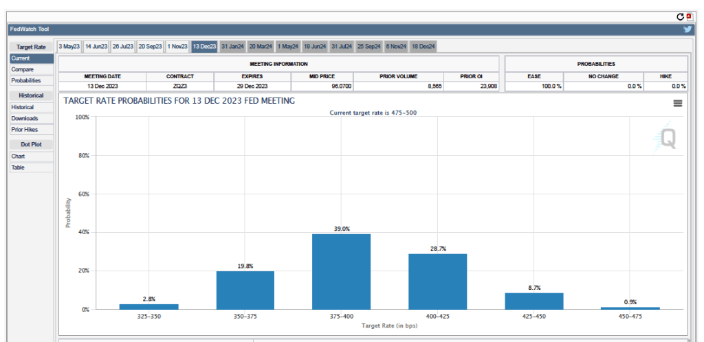
The chart shows six possible ranges for the federal funds rate after the FOMC’s last meeting in December 2023. Note that the ranges are given in basis points (bps). Each basis point is one hundredth of a percentage point. So, for instance, the range of 375-400 equals a range of 3.75 percent to 4.00 percent. The numbers at the top of the blue rectangles represent the probability that investors place on that range occurring after the FOMC’s December meeting. So, for instance, the probability of the federal funds rate target being 4.00 percent to 4.25 percent is 28.7 percent. The sum of the probabilities equals 1.
Note that the highest target range given on the chart is 4.50 percent to 4.75 percent. In other words, investors in financial markets are assigning a probability of zero to an outcome that the dot plot shows 17 of 18 FOMC members believe will occur: A federal funds rate greater than 5 percent. This is a striking discrepancy between what the FOMC is announcing it will do and what financial markets think the FOMC will actually do.
In other words, financial markets are indicating that actual Fed policy for the remainder of 2023 will be different from the policy that the Fed is indicating it intends to carry out. Why don’t financial markets believe the Fed? It’s impossible to say with certainty but here are two possibilities:
- Markets may believe that the Fed is underestimating the likelihood of an economic recession later this year. If an economic recession occurs, markets assume that the FOMC will have to pivot from increasing its target for the federal funds rate to cutting its target. Markets may be expecting that the banks will cut back more on the credit they offer households and firms as the banks prepare to deal with the possibility that substantial deposit outflows will occur. The resulting credit crunch would likely be enough to push the economy into a recession.
- Markets may believe that members of the FOMC are reluctant to publicly indicate that they are prepared to cut rates later this year. The reluctance may come from a fear that if households, investors, and firms believe that the FOMC will soon cut rates, despite continuing high inflation rates, they may cease to believe that the Fed intends to eventually bring the inflation back to its 2 percent target. In Fed jargon, expectations of inflation would cease to be “anchored” at 2 percent. Once expectations become unanchored, higher inflation rates may become embedded in the economy, making the Fed’s job of bringing inflation back to the 2 percent target much harder.
In late December, we can look back and determine whose forecast of the federal funds rate was more accurate–the market’s or the FOMC’s.
Is the Banking Crisis Over? Some Banks Don’t Seem to Think So

Bank borrowing from the Fed. Figure from the Federal Reserve Bank of St. Louis FRED data set.
Discount loans were the Fed’s original policy tool. As we discuss in Macroeconomics, Chapter 15, Section 15.4 (Economics, Chapter 25, Section 25.4) and in Money, Banking, and the Financial System, Chapter 13, Section 13.1, Congress established the Fed to serve as a lender of last resort making loans to banks that were having temporary liquidity problems because depositors were withdrawing more funds than the bank could meet from its own cash holdings. Discount loans were intended to be short term, often overnight, and were to be made only to healthy banks that were solvent—the value of the banks’ assets were greater than the value of their liabilities—and that could pledge short-term business loans (called at the time “real bills”) as collateral.
Today, healthy banks with temporary liquidity needs can request a loan through the Fed’s discount window (an antique term dating from the early years of the system when the loans were literally made at a specific window at each regional Fed bank) from the Fed’s primary credit facility, or standing lending facility. Over the years, the importance of discount loans declined. The establishment of the Federal Deposit Insurance Corporation (FDIC) in 1934 reassured households and businesses that held deposits below the insurance limit that they did not need to withdraw their deposits at the first sign of trouble with their local bank. As a result, after the establishment of the FDIC few banks experienced runs.
In addition, the development of the federal funds market gave banks another source of short-term credit. Because the federal funds rate is typically lower than the interest rate (the discount rate) that the Fed charges on discount loans, most banks find borrowing in the federal funds market preferrable to borrowing at the Fed’s discount window. As banks’ use of discount loans declined, many banks were afraid that going to the discount window would be seen by depositors and investors as a sign the bank was in financial trouble. This stigma was an additional reason that most banks avoided borrowing at the discount window.
As the figure shows, in the years leading up to the Great Financial Crisis, the volume of discount loans had dwindled to very low levels. After a surge in discount borrowing following the failure of the Lehman Brothers investment bank in September 2008, discount borrowing gradually fell back to low levels. A smaller surge in discount borrowing occurred in the spring of 2020 at the beginning of the Covid–19 pandemic in the United States. Discount borrowing quickly declined during the following months.
The failure of Silicon Valley Bank (SVB) on March 10 and Signature Bank on March 12 pushed the volume of discount loans to record levels, as shown by the vertical line at the far right of the figure. The values in the figure include three types of loans:
- Primary credit, which are traditional discount loans.
- Other credit extensions, which are loans from Federal Reserve District Banks to the FDIC to fund so-called bridge banks established by the FDIC to operate SVB and Signature Bank until either purchasers can be found for the banks or their assets can be sold and the banks permanently closed.
- Loans under the Fed’s Bank Term Funding Program, which are loans the Fed has made under this new facility established on March 12. The loans are secured by the borrowing banks’ holdings of Treasury and mortgage-backed securities.
The data underlying the figure come from the Fed’s H.4.1 statistical release, “Factors Affecting Reserve Balances of Depository Institutions and Condition Statement of Federal Reserve Banks,” which can be found here.
Which banks are doing this borrowing? To avoid stigma, the Fed doesn’t release the names of the banks for two years, but, presumably, regional banks, such as First Republic Bank, that have been experiencing substantial depositor withdrawals are doing so. (First Republic has publicly announced that it is borrowing from the Fed.) The amounts borrowed are so large, however, that it appears that a significant number of banks are either in need of liquidity or are preparing to be able to meet waves of deposit withdrawals should they occur.
Whether the banking crisis that began with the failure of SVB is largely over is unclear at this point, but the managers of some banks are preparing in case the crisis continues.
The FOMC Splits the Difference with a 0.25 Percentage Point Rate Increase
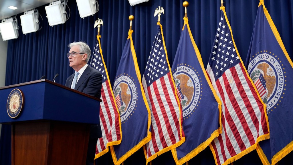
Photo from the Wall Street Journal.
At the conclusion of its meeting today (March 22, 2023), the Federal Reserve’s Federal Open Market Committee (FOMC) announced that it was raising its target for the federal funds rate from a range of 4.50 percent to 4.75 percent to a range of 4.75 percent to 5.00 percent. As we discussed in this recent blog post, the FOMC was faced with a dilemma. Because the inflation rate had remained stubbornly high at the beginning of this year and consumer spending and employment had been strongly increasing, until a couple of weeks ago, financial markets and many economists had been expecting a 0.50 percentage point (or 50 basis point) increase in the federal funds rate target at this meeting. As the FOMC noted in the statement released at the end of the meeting: “Job gains have picked up in recent months and are running at a robust pace; the unemployment rate has remained low. Inflation remains elevated.”
But increases in the federal funds rate lead to increases in other interest rates, including the interest rates on the Treasury securities and mortgage-backed securities that most banks own. On Friday, March 10, the Federal Deposit Insurance Corporation (FDIC) was forced to close the Silicon Valley Bank (SVB) because the bank had experienced a deposit run that it was unable to meet. The run on SVB was triggered in part by the bank taking a loss on the Treasury securities it sold to raise the funds needed to cover earlier deposit withdrawals. The FDIC also closed New York-based Signature Bank. San Francisco-based First Republic Bank experienced substantial deposit withdrawals, as we discussed in this blog post. In Europe, the Swiss bank Credit Suisse was only saved from failure when Swiss bank regulators arranged for it to be purchased by UBS, another Swiss bank. These problems in the banking system led some economists to urge that the FOMC keep its target for the federal funds rate unchanged at today’s meeting.
Instead, the FOMC took an intermediate course by raising its target for the federal funds rate by 0.25 percentage point rather than by 0.50 percentage point. In a press conference following the announcement, Fed Chair Jerome Powell reinforced the observation from the FOMC statement that: “Recent developments are likely to result in tighter credit conditions for households and businesses and to weigh on economic activity, hiring, and inflation.” As banks, particularly medium and small banks, have lost deposits, they’ve reduced their lending. This reduced lending can be a particular problem for small-to medium-sized businesses that depend heavily on bank loans to meet their credit needs. Powell noted that the effect of this decline in bank lending on the economy is the equivalent of an increase in the federal funds rate.
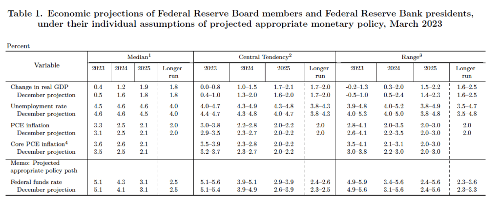
The FOMC also released its Summary of Economic Projections (SEP). As Table 1 shows, committee members’ median forecast for the federal funds rate at the end of 2023 is 5.1 percent, indicating that the members do not anticipate more than a single additional 0.25 percentage point increase in the target for the federal funds rate. The members expect a significant increase in the unemployment rate from the current 3.6 percent to 4.5 percent at the end of 2023 as increases in interest rates slow down the growth of aggregate demand. They expect the unemployment rate to remain in that range through the end of 2025 before declining to the long-run rate of 4.0 percent in later years. The members expect the inflation rate as measured by the personal consumption (PCE) price index to decline from 5.4 percent in January to 3.3 percent in December. They expect the inflation rate to be back close to their 2 percent target by the end of 2025.
Sheila Bair Would Have Voted “No” on SVB

Photo from Washington College via Wikipedia.
Sheila Bair served as chair of the Federal Deposit Insurance Corporation (FDIC) from 2006 to 2011. This week, she was interviewed on the Wall Street Journal’s “Free Expression” podcast. She states that she had still been chair of the FDIC she would have been against the decision on Sunday, March 12, 2023, to declare that Silicon Valley Bank (SVB) as being systemically important. The declaration formed the basis of the decision by the FDIC, the Federal Rerserve, and the Treasure that SVB’s customers with deposits above the normal $250,000 insurance limit would be allowed to withdraw all their funds beginning Monday morning.
She argues that it would have been better to have followed the FDIC’s usual procedure of allowing insured depositors to withdraw their funds and declaring a “dividend” that would have allowed withdrawal of 50 percent of uninsured deposits. As SVB’s assets were sold, uninsured depositors would be able to make additional withdrawals, although because the value of the assets would likely be less than the value of the deposits, uninsured depositors would suffer some losses.
She believes that SVB’s problems were the result of poor management and she doubts that the bank’s uninsured depositors suffering losses would have led to runs on the deposits of other regional banks.
The wide-ranging interview is well worth listening to in full. The podcast can be found here.
Somewhere J. P. Morgan Is Smiling: The Attempt by Large Banks to Support First Republic Bank
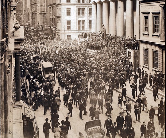
Wall Street during the Panic of 1907. (Photo from the New York Public Library via Federal Reserve History.)
The collapse of Silicon Valley Bank (SVB) on Friday, March 10 highlighted two potential sources of instability in the U.S. commercial banking system: (1) The risk that depositors with more than the Federal Deposit Insurance Corporation (FDIC) insurance deposit limit of $250,000 in their accounts may withdraw their deposits leading to liquidity problems in the banks experiencing the withdrawals; and (2) The losses many banks have taken on their Treasury and mortgage-backed securities as interest rates have risen. (We discuss SVB in this post and banks’ losses on their security holdings in this post.) The sources of instability are related in that the losses on their security holdings may cause banks to have difficulty obtaining the funds to meet deposit withdrawals.
Note that, although the FDIC, the Federal Reserve, and the Treasury guaranteed all deposits in SVB and in Signature Bank (which was closed on Sunday, March 1), the FDIC insurance limit of $250,000 per deposit, per bank remains in effect for all other banks.
The banks most at risk for large deposit outflows are the regional banks. In terms of size, regional banks stand intermediate between the large national banks, like JP Morgan Chase and Bank of America, and small community banks. Depositors seem reassured that the large national banks have sufficient capital to withstand deposit outflows. The small community banks mainly hold retail deposits—deposits made by households and local businesses—that are typically below the $250,000 FDIC deposit limit.
On Thursday, March 16, First Republic Bank seemed to be the regional bank at most risk. Over the previous several days it experienced an outflow of billions of dollars in deposits. The Fed’s new Bank Term Funding Program (BTFP) made it possible for First Republic to borrow against its Treasury and mortgage-backed securities holdings—rather than selling the securities—to meet deposit outflows. Investors were not reassured, however, that using the BFTP would be sufficient to meet First Republic’s funding needs. The bank’s stock fell sharply on Wednesday and again on Thursday morning. S&P reduced its rating of the bank’s bonds to junk status. (We discuss bond ratings in an Apply the Concept in Macroeconomics, Chapter 6, Section 6.2 (Economics, Chapter 8, Section 8.2) and, at greater length, in Money, Banking, and the Financial System, Chapter 5, Section 5.1.)
According to an article in the Wall Street Journal, on Thursday morning: “The biggest banks in the U.S. are discussing a joint rescue of First Republic Bank that could include a sizable capital infusion to shore up the beleaguered lender .… The rescue would be an extraordinary effort to protect the entire banking system from widespread panic by turning First Republic into a firewall.” Among the banks participating in the plan are JP Morgan Chase, Well Fargo, Citigroup, and Bank of America. Because many large depositors had been switching their deposits from regional banks like First Republic to large banks, according to the article, the resuce plan would include the large banks making deposits in First Republic, thereby indirectly returning some of the deposits that First Republic had lost.
The banks involved in the rescue plan were apparently consulting with the Federal Reserve and the Treasury. Because this plan involved private banks attempting to help another private bank deal with deposit outflows, it was reminiscent of the actions of the bank clearing houses that operated in major cities before the Federal Reserve began operations in 1914.
Under this system, all the largest banks in a city were typically members of the clearing house, as were many midsize banks. The clearing houses had the ability to advance funds to meet the short-run liquidity needs of members. In effect, the clearing houses were operating in a way similar to the Fed’s extension of discount loans. Although the clearing houses were unable to stop bank panics, there is evidence that they were helpful in reducing deposit outflows from member banks. The famous financier J. P. Morgan was the most influential figure in the New York Clearing House during the early 1900s. This article on the Panic of 1907 discusses the role of Morgan and the New York Clearing House. A discussion of how the actions of the New York Clearing House compare with the actions of a government central bank, like the Fed, can be found here.
The Fed’s Latest Dilemma: The Link between Monetary Policy and Financial Stability
AP photo from the Wall Street Journal
Congress has given the Federal Reserve a dual mandate of high employment and price stability. In addition, though, as we discuss in Macroeconomics, Chapter 15, Section 15.1 (Economics, Chapter 25, Section 25.1) and at greater length in Money, Banking, and the Financial System, Chapter 15, Section 15.1, the Fed has other goals, including the stability of financial markets and institutions.
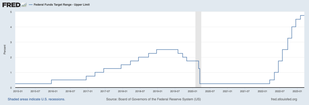
Since March 2022, the Fed has been rapidly increasing its target for the federal funds rate in order to slow the growth in aggregate demand and bring down the inflation rate, which has been well above the Fed’s target of 2 percent. (We discuss monetary policy in a number of earlier blog posts, including here and here, and in podcasts, the most recent of which (from February) can be found here.) The target federal funds rate has increased from a range of 0 percent to 0.25 percent in March 2022 to a range of 4.5 percent to 4.75 percent. The following figure shows the upper range of the target for the federal funds rate from January 2015 through March 14, 2023.
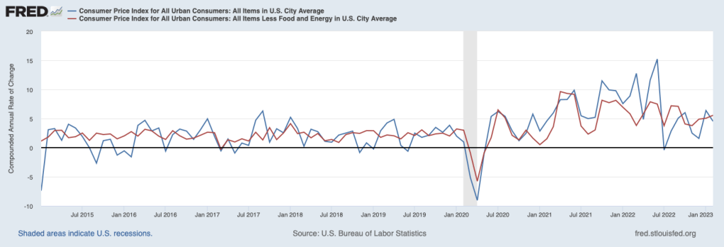
This morning (Tuesday, March 14, 2023), the Bureau of Labor Statistics (BLS) released its data on the consumer price index for February. The following figure show inflation as measured by the percentage change in the CPI from the same month in the previous year (which is the inflation measurement we use most places in the text) and as the percentage change in core CPI, which excludes prices of food and energy. (The inflation rate computed by the percentage change in the CPI is sometimes referred to as headline inflation.) The figure shows that although inflation has slowed somewhat it is still well above the Fed’s 2 percent target. (Note that, formally, the Fed assesses whether it has achieved its inflation target using changes in the personal consumption expenditures (PCE) price index rather than using changes in the CPI. We discuss issues in measuring inflation in several blog posts, including here and here.)
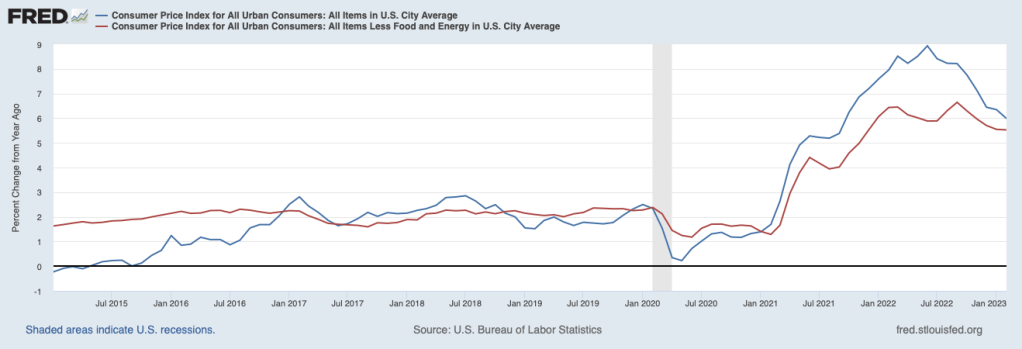
One drawback to using the percentage change in the CPI from the same month in the previous year is that it reduces the weight of the most recent observations. In the figure below, we show the inflation rate measured by the compounded annual rate of change, which is the value we would get for the inflation rate if that month’s percentage change continued for the following 12 months. Calculated this way, we get a somewhat different picture of inflation. Although headline inflation declines from January to February, core inflation is actually increasing each month from November 2022 when, it equaled 3.8 percent, through February 2023, when it equaled 5.6 percent. Core inflation is generally seen as a better indicator of future inflation than is headline inflation.
The February CPI data are consistent with recent data on PCE inflation, employment growth, and growth in consumer spending in that they show that the Fed’s increases in the target for the federal funds rate haven’t yet caused a slowing of the growth in aggregate demand sufficient to bring the inflation back to the Fed’s target of 2 percent. Until last week, many economists and Wall Street analysts had been expecting that at the next meeting of the Fed’s Federal Open Market Committee (FOMC) on March 21 and 22, the FOMC would raise its target for the federal funds rate by 0.5 percentage points to a range of 5.0 percent to 5.25 percent.
Then on Friday, the Federal Deposit Insurance Corporation (FDIC) was forced to close the Silicon Valley Bank (SVB). As the headline on a column in the Wall Street Journal put it “Fed’s Tightening Plans Collide With SVB Fallout.” That is, the Fed’s focus on price stability would lead it to continue its increases in the target for the federal funds rate. But, as we discuss in this post from Sunday, increases in the federal funds rate lead to increases in other interest rates, including the interests rates on the Treasury securities, mortgage-backed securities, and other securities that most banks own. As interest rates rise, the prices of long-term securities decline. The run on SVB was triggered in part by the bank taking a loss on the Treasury securities it sold to raise the funds needed to cover deposit withdrawals.
Further increases in the target for the federal funds rate could lead to further declines in the prices of long-term securities that banks own, which might make it difficult for banks to meet deposit withdrawals without taking losses on the securities–losses that have the potential to make the banks insolvent, which would cause the FDIC to seize them as it did SVB. The FOMC’s dilemma is whether to keep the target for the federal funds rate unchanged at its next meeting on March 21 and 22, thereby keeping banks from suffering further losses on their bond holdings, or to continue raising the target in pursuit of its mandate to restore price stability.
Some economists were urging the FOMC to pause its increases in the target federal funds rate, others suggested that the FOMC increase the target by only 0.25 percent points rather than by 0.50 percentage points, while others argued that the FOMC should implement a 0.50 increase in order to make further progress toward its mandate of price stability.
Forecasting monetary policy is a risky business, but as of Tuesday afternoon, the likeliest outcome was that the FOMC would opt for a 0.25 percentage point increase. Although on Monday the prices of the stocks of many regional banks had fallen, during Tuesday the prices had rebounded as investors appeared to be concluding that those banks were not likely to experience runs like the one that led to SVB’s closure. Most of these regional banks have many more retail deposits–deposits made be households and small local businesses–than did SVB. Retail depositors are less likely to withdraw funds if they become worried about the solvency of a bank because the depositors have much less than $250,000 in their accounts, which is the maximum covered by the FDIC’s deposit insurance. In addition, on Sunday, the Fed established the Bank Term Funding Program (BTFP), which allows banks to borrow against the holdings of Treasury and mortgage-back securities. The program allows banks to meet deposit withdrawals by borrowing against these securities rather than by having to sell them–as SVB did–and experience losses.
On March 22, we’ll find out how the Fed reacts to the latest dilemma facing monetary policy.
3/13/23 Podcast – Authors Glenn Hubbard & Tony O’Brien discuss the collapse of SVB in the context of a classic bank run. Is it? Listen & find out.
Join authors Glenn Hubbard and Tony O’Brien as they review the collapse of Silicon Valley Bank (SVB) in the context of a classic bank run. What lessons can be learned to avoid other bank collapses in this unchartered economic territory? Will this become a contagion? Or, is it simply an example of a bank searching for additional return in an uncertain economic world? Our discussion covers these points but you can also check for updates on our blog post that can be found HERE.
