Image generated by ChatGPT
Recently, Rustam Jamilov of the University of Oxford posted the following figure to X, noting that: “A new paper shows that the release of Pirates of the Caribbean was associated with a 38% decline in real-world piracy incidents. The lives saved by Disney are staggering.”
A recent article in the New York Times had the headline “Get a Dog, Live Longer.” The article stated that: “Research dating back decades has found that people who own pets, especially dogs, tend to be healthier than people who don’t.” A “large review of studies published in 2019 found that owning a dog was associated with a 24 percent lower risk of dying from all causes over the course of 10 years.”
An article in the Washington Post had the headline “Drink Coffee to Prevent Dementia? It’s Not So Far-Fetched.” The article reports on a study in which “The researchers analyzed data from more than 131,000 people over multiple decades.” The key finding of the study was that “Those who regularly drank caffeinated coffee had an 18 percent lower risk [of developing dementia] compared to people who drank little or none. Regular coffee drinkers also performed better on some cognitive tests and were less likely to report mental decline.”
All three of these cases involve observational studies, rather than experiments. In experiments, researchers assign some randomly selected people to a treatment group and other people to a control group. If you wanted to test the effect of having a dog on a person’s health, you could give a dog to a randomly selected group of people—the treatment group—and assign another randomly selected group of people to remain without a dog—the control group. Then you would follow both groups for a period of years and see if there was any difference in health outcomes between the people with a dog and those without a dog.
As this example indicates, experiments can be an impractical way to test a hypothesis. So instead, researchers often follow a group of people over time and then look for correlations between their activities—having a dog or drinking coffee, for example—and their life outcomes: Are people who engage in these activities healthier, happier, more likely to be married, have higher incomes, and so on. Observational studies can generate correlations between two variables, but it’s not clear if they establish causation—does owning a dog cause you to be healthier.
Some correlations are obvious nonsense. Rustam Jamilov is joking when he pretends that, because a decline in piracy in the real world followed the release of the first Pirates of the Caribbean movie, releasing the movie reduced piracy. In Chapter 6 of Money, Banking, and the Financial System we discuss the nonsense correlation discovered by Leonard Koppett when he noticed that—for a period of 11 years—which conference the winner of the National Football League’s Super Bowl was from was correlated with the performance of the stock market in the following year.
The claims that owning a dog or drinking coffee might improve your health seem more plausible because you can think of reasonable causal mechanisms. For instance, if you own a dog you might be more likely to take long walks, which may improve your health. And there may be some attribute of caffeine that makes coffee drinkers less likely to suffer from dementia.
The problem is that because people in an observational study aren’t randomly assigned to engage in the activity being studied—owning a dog or drinking coffee—we can’t be sure if people engaging in these activities differ systematically from those who don’t. As the article on the health benefits of dogs points out: “Dog owners tend to be younger and richer than non-owners, characteristics that correspond with better health.” Observational studies generally fail to control for these confounding factors, making it more difficult to determine if the correlations they find are causal.

Image created by ChatGPT
A famous example of concluding that a correlation was causal when it likely wasn’t comes from the Nurses’ Health Study (NHS), which followed more than 30,000 postmenopausal nurses beginning in 1976. The nurses who used hormone therapies were more than 40 percent less likely to develop coronary heart disease. This correlation was believed to be causal, which resulted in many more postmenopausal women being proscribed hormone therapies.
This conclusion was reversed by the Women’s Health Initiative (WHI), which was conducted in the 1990s and randomly assigned women to receive hormone therapy or a placebo. The women receiving the hormone therapy turned out to be more likely to experience coronary problems. Part of the explanation appears to be that the nurses in the NHS who used the hormone therapy were already healthier in some respects, such as having lower weight and lower blood pressure, than the nurses who did not use the hormone therapy. (Note: The findings in this area complex and are still being debated, so don’t take our brief summary as a definitive account!)

Image created by ChatGTP
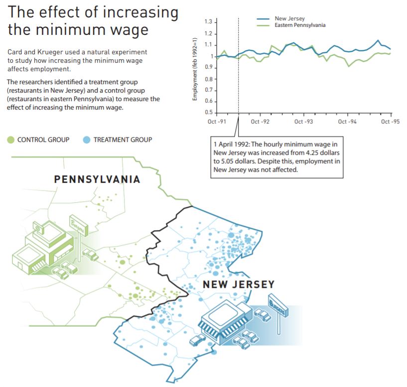
In recent years, economists have often used natural experiments to attempt to identify causal results from observational studies. With a natural experiment, economists identify some variable of interest—say, an increase in the minimum wage—that has changed for one group of people—say, fast-food workers in one state—while remaining unchanged for another similar group of people—say, fast-food workers in a neighboring state. Researchers can draw an inference about the effects of the change by looking at the difference between the outcomes for the two groups. In this example, the difference between changes in employment at fast-food restaurants in the two states can be used to measure the effect of an increase in the minimum wage.
In a famous study of the effect of the minimum wage on employment in the fast food industry published in 1994 in the American Economic Review, David Card of the University of California, Berkeley and the late Alan Krueger of Princeton University pioneered the use of natural experiments. In that study, Card and Krueger analyzed the effect of the minimum wage on employment in fast-food restaurants by comparing what happened to employment in New Jersey when it raised the state minimum wage from $4.25 to $5.05 per hour with employment in eastern Pennsylvania where the minimum wage remained unchanged. They found that, contrary to the usual analysis that increases in the minimum wage lead to decreases in the employment of unskilled workers, employment of fast-food workers in New Jersey actually increased relative to employment of fast-food workers in Pennsylvania. Card shared the 2021 Nobel Prize in Economics with Joshua Angrist of the Massachusetts Institute of Technology; and Guido Imbens of Stanford University in part for his work using natural experiments.
The following graphic from Nobel Prize website summarizes the study. (Note that not all economists have accepted the results of Card and Krueger’s study. We briefly summarize the debate over the effects of the minimum wage in Microeconomics and Economics, Chapter 4, Section 4.3.)
So, attempting to draw causal inferences from observational studies is hard. Having a dog or drinking coffee may not actually improve your health.
But why take chances? Adopt a dog!