Is the refrigerator above different from the refrigerator below?
Consumer Reports is a magazine and web site devoted to product reviews. Their November-December 2024 issue noted something unusual about the two GE refrigerators shown above. (The images are from the geappliances.com web site.) At the time the issue was printed, the first refrigator above had a price of $2,300 and the second refrigerator had a price of $1,300: Consumer Reports notes that:
“These look-alike fridges offer equally impressive performance, have the same interior features … and are from the same brand. So why the $1,000 price difference? We don’t know.”
(Note: GE referigators, and many other products branded with the GE name are no longer produced by the General Electric company, which dates back to 1892 and was co-founded by Thomas Edison. Today, GE is primarily an aerospace company and GE appliances are produced by the Chinese-owned Haier Smart Home Company.)
If we assume that Consumer Reports is correct and the two refrigerators are identical, what strategy is the firm pursuing by charging different prices for the same product? As we discuss in Microeconomics, Chapter 15, Section 15.5 firms can increase their profits by practicing price discrimination—charging different prices to different customers. To pursue a strategy of price discrimination the firm needs to be able to divide up—or segment—the market for its refrigerators.
Firms sometimes use a high price to signal quality. The old saying “you get what you pay for” can lead some consumers to expect that when comparing two similar goods, such as two models of refrigerators, the one with the higher price also has higher quality. In the appliance section of a large store, such as Lowe’s or the Home Depot, or online at Amazon or another site, you will have a wide variety of refrigerators to choose from. You may have trouble evaluating the features each model offers and be unable to tell whether a particular model is likely to be more or less reliable. So, if you are choosing between the two GE models shown above, you may decide to choose the one with the higher price because the higher price may indicate that the components used are of higher quality.
In this case, GE may be relying on a segmentation in the market between consumers who carefully research the features and the quality of the refrigerators that different firms offer for sale and those consumers don’t. The consumers who do careful research and are aware of all the features of each model may be more sensitive to the price and, therefore, have a high price elasticity of demand. The consumers who haven’t done the research may be relying on the price as a signal of quality and, therefore, have a lower price elasticty of demand.
If what we have just outlined was the firm’s strategy for increasing profit by charging different prices for two models that are, apparently, either identical or very similar, it doesn’t seem to have worked. Note that the model shown in the first photo above is the one that had a price of $2,300 when Consumer Reports wrote about it, but now has a price of $1,154.40. The model shown in the second photo had a price of $1,300, but now has a price of $1,399.00. In other words, the model that had the lower price now has the higher price and the model that had the higher price now has the lower price.
What happened between the time the issue of Consumer Reports published and now? We might conjecture that there are few consumers who would be likely to pay $1,000 more for a refrigator that seems to have the same features as another model from the same company. In other words, segmenting consumers in this way seems unlikely to succeed. Why, though, the firm decided to make its formerly higher-price model its lower-price model, is difficult to explain without knowing more about the firm’s pricing strategy.
Nvidia’s headquarters in Santa Clara, California. (Photo from nvidia.com)
Nvidia was founded in 1993 by Jensen Huang, Chris Malachowsky, and Curtis Priem, electrical engineers who started the company with the goal of designing computer chips that would increase the realism of images in video games. The firm achieved a key breakthrough in 1999 when it invented the graphics processing unit, or GPU, which it marketed under the name GeForce256. In 2001, Microsoft used a Nvidia chip in its new Xbox video game console, helping Nvidia to become the dominant firm in the market for GPUs.
The technology behind GPUs has turned out to be usable not just for gaming, but also for powering AI—artificial intelligence—software. The market for Nvidia’s chips exploded witth technology giants Google, Microsoft, Facebook and Amazon, as well as many startups ordering large quantites of Nvidia’s chips.
By 2016, Nvidia CEO Jen-Hsun Huang could state in an interview that: “At no time in the history of our company have we been at the center of such large markets. This can be attributed to the fact that we do one thing incredibly well—it’s called GPU computing.” Earlier this year, an article in the Economist noted that: “Access to GPUs, and in particular those made by Nvidia, the leading supplier, is vital for any company that wants to be taken seriously in artificial intelligence (AI).”
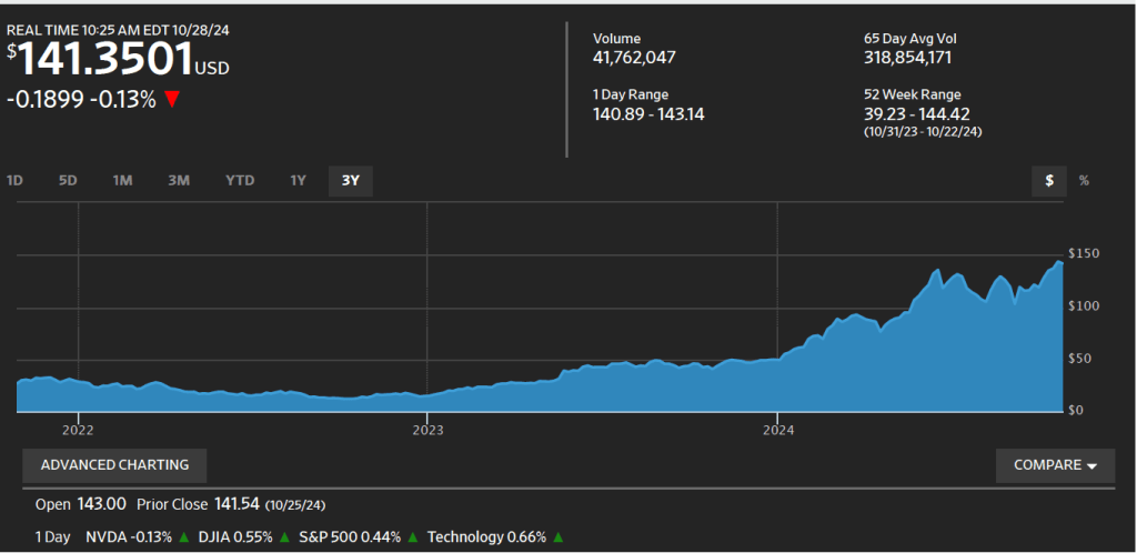
Nvidia’s success has been reflected in its stock price. When Nvidia became a public company in 1999 by undertaking an initial public offering (IPO) of stock, a share of the firm’s stock had a price of $0.04, adjusted for later stock splits. The large profits Nvidia has been earning in recent years have caused its stock price to rise to more than $140 dollars a share.
(With a stock split, a firm reduces the price per share of its stock by giving shareholders additional shares while holding the total value of the shares constant. For example, in June of this year Nvidia carried out a 10 for 1 stock split, which gave shareholders nine shares of stock for each share they owned. The total value of the shares was the same, but each share now had a price that was 10 percent of its price before the split. We discuss the stock market in Microeconomics, Chapter 8, Section 8.2, Macroeconomics, Chapter 6, Section 6.2, and Economics, Chapter 8, Section 8.2.)
The following figure from the Wall Street Journal shows the sharp increase in Nvidia’s stock price over the past three years as AI has become an increasingly important part of the economy.
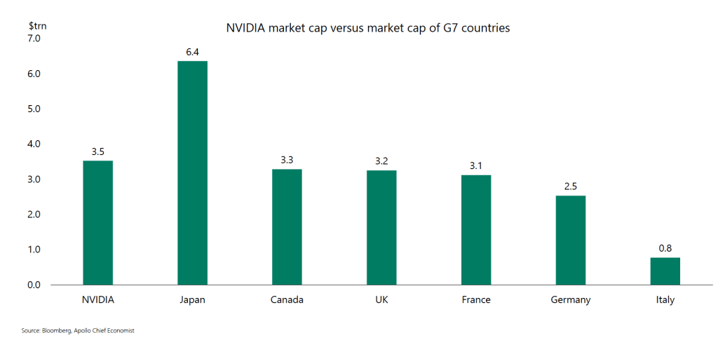
Nvidia’s market capitalization (or market cap)—the total value of all of its outstanding shares of stock—is $3.5 trillion. How large is that? Torsten Sløk, the chief economist at Apollo, an asset management firm, has noted that, as shown in the following figure, Nvidia’s market cap is larger than the total market caps—the total value of all the publicly traded firms—in five large economies.
Can Nvidia’s great success continue? Will it be able to indefinitely dominate the market for AI chips? As we noted in Apply the Concept “Do Large Firms Live Forever?” in Microeconomics Chapter 14, in the long run, even the most successful firms eventually have their positions undermined by competition. That Nvidia has a larger stock market value than the total value of all the public companies in Germany or the United Kingdom is extraordinary and seems impossible to sustain. It may indicate that investors have bid up the price of Nvidia’s stock above the value that can be justified by a reasonable forecast of its future profits.
There are already some significant threats to Nvidia’s dominant position in the market for AI chips. GPUs were originally designed to improve computer displays of graphics rather than to power AI software. So, one way of competing with Nvidia that some startups are trying to exploit is to design chips specifically for use in AI. It’s also possible that larger chips may make it possible to use fewer chips than when using GPUs, possibly reducing the total cost of the chips necessary to run sophisticated AI software. In addition, existing large technology firms, such as Amazon and Microsoft, have been developing chips that may be able to compete with Nvidia.
As with any firm, Nvidia’s continued success requires it to innovate sufficiently to stay ahead of the many competitors that would like to cut into the firm’s colossal profits.
Image generated by GTP-4o of someone searching online for a job
It’s become clear during the past few years that most people really, really, really don’t like inflation. Dating as far back as the 1930s, when very high unemployment rates persisted for years, many economists have assumed that unemployment is viewed by most people as a bigger economic problem than inflation. Bu the economic pain from unemployment is concentrated among those people who lose their jobs—and their families—although some people also have their hours reduced by their employers and in severe recessions even people who retain their jobs can be afraid of being laid off.
Although nearly everyone is affected by an increase in the inflation rate, the economic losses are lower than those suffered by people who lose their jobs during a period in which it may difficult to find another one. In addition, as we note in Macroeconomics, Chapter 9, Section 9.7 (Economics, Chapter 19, Section 19.7), that:
“An expected inflation rate of 10 percent will raise the average price of goods and services by 10 percent, but it will also raise average incomes by 10 percent. Goods and services will be as affordable to an average consumer as they would be if there were no inflation.”
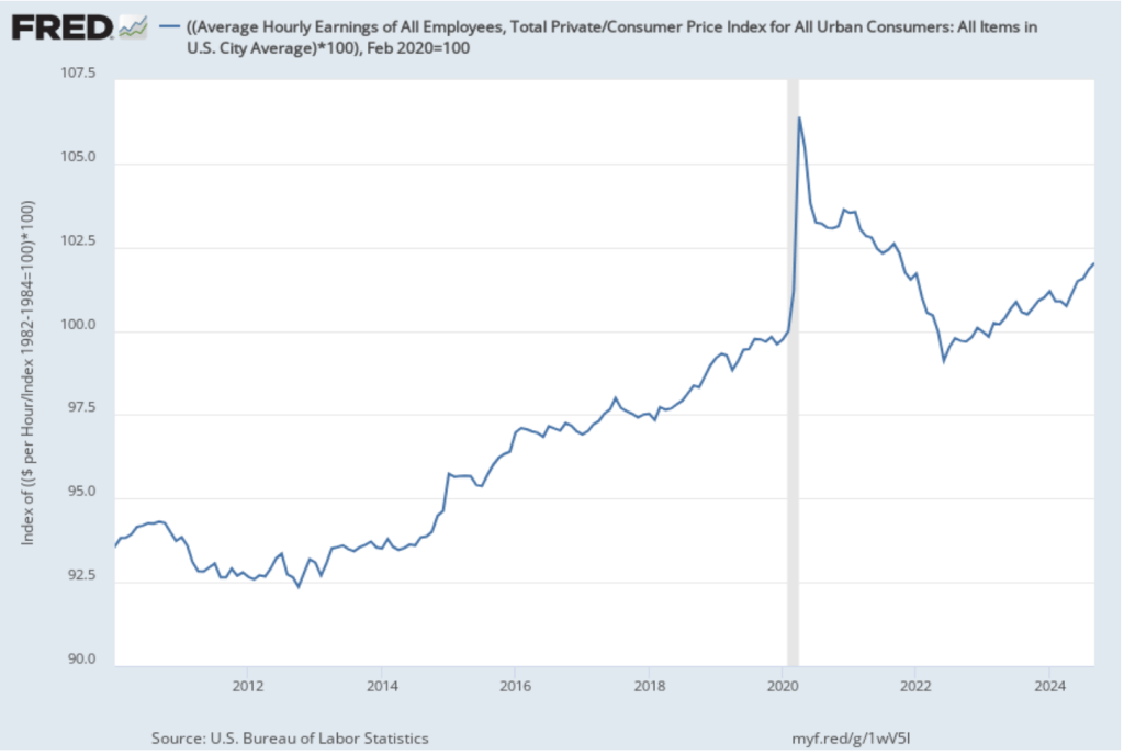
In other words, inflation affects nominal variables, but over the long run inflation won’t affect real variables such as the real wage, employment, or the real value of output. The following figure shows movements in real wages from January 2010 through September 2024. Real wages are calculated as nominal average hourly earnings deflated by the consumer price index, with the value for February 2020—the last month before the effects of the Covid pandemic began affecting the United States—set equal to 100. Measured this way, real wages were 2 percent higher in September 2024 than in February 2020. (Although note that real wages were below where they would have been if the trend from 2013 to 2020 had continued.)
Although increases in wages do keep up with increases in prices, many people doubt this point. In Chapter 17, Section 17.1, we discuss a survey Nobel Laurete Rober Shiller of Yale conducted of the general public’s views on inflation. He asked in the survey how “the effect of general inflation on wages or salary relates to your own experience or your own job.” The most populat response was: “The price increase will create extra profifs for my employer, who can now sell output for more; there will be no increase in my pay. My employer will see no reason to raise my pay.”
Recently, Stefanie Stantcheva of Harvard conducted a survey similar to Schiller’s and received similar responses:
“If there is a single and simple answer to the question ‘Why do we dislike inflation,’ it is because many individuals feel that it systematically erodes their purchasing power. Many people do not perceive their wage increases sufficiently to keep up with inflation rates, and they often believe that wages tend to rise at a much slower rate compared to prices.”
A recent working paper by Joao Guerreiro of UCLA, Jonathon Hazell of the London School of Economics, Chen Lian of UC Berkeley, and Christina Patterson of the University of Chicago throws additional light on the reasons that people are skeptical that once the market adjusts, their wages will keep up with inflation. Economists typically think of the real wage as adjusting to clear the labor market. If inflation temporarily reduces the real wage, the nominal wage will increase to restore the market-clearing value of the real wage.
But the authors of thei paper note that, in practice, to receive an increase in your nominal wage you need to either 1)ask your employer to increase your wage, or 2) find another job that pays a higher nominal wage. They note that both of these approachs result in “conflict”: “We argue that workers must take costly actions (‘conflict’) to have nominal wages catch up with inflation, meaning there are welfare costs even if real wages do not fall as inflation rises.” The results of a survey they undertook revealed that:
“A significant portion of workers say they took costly actions—that is, they engaged in conflict—to achieve higher wage growth than their employer offered. These actions include having tough conversations with employers about pay, partaking in union activity, or soliciting job offers.”
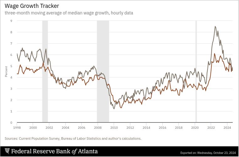
Their result is consistent with data showing that workers who switch jobs receive larger wage increases than do workers who remain in their jobs. The following figure is from the Federal Reserve Bank of Cleveland and shows the increase in the median nominal hourly wage over the previous year for workers who stayed in their job over that period (brown line) and for workers who switched jobs (gray line).
Job switchers consistently earn larger wage increases than do job stayers with the difference being particularly large during the high inflation period of 2022 and 2023. For instance, in July 2022, job switchers earned average wage increases of 8.5 percent compared with average increases of 5.9 percent for job stayers.
The fact that to keep up with inflation workers have to either change jobs or have a potentially contentious negotiation with their employer provides another reason why the recent period of high inflation led to widespread discontent with the state of the U.S. economy.
Daron Acemoglu and Simon Johnson (Credit: Acemoglu, Adam Glanzman; Johnson, courtesy of MIT, from news.mit.edu)
James Robinson (photo from news.uchicago.edu)
Many economic studies have a relatively limited objective. For instance, estimating the price elasticity of demand for soda in order to determine the incidence of a soda tax. Or estimating a Keynesian fiscal policy multiplier in order to determine the effects of a change in federal spending or taxes. (We consider the first topic in Microeconomics, Chapter 6, and the second topic in Macroeconomics, Chapter 16.)
Other economic studies consider much broader questions, such as why are some countries rich and other countries poor? As the late Nobel laureate Robert Lucas once wrote: “The consequences for human welfare involved in questions like these are simply staggering: Once one starts to think about them, it is hard to think about anything else.”
Today, the Royal Swedish Academy of Sciences awarded the 2024 Nobel Prize in Economic Sciences to Daron Acemoglu and Simon Johnson of MIT, and to James Robinson of the University of Chicago for “for studies of how institutions are formed and affect prosperity.” Acemoglu, Johnson, and Robinson (AJR) have published work highlighting the key importance of a country’s institutions in explaining whether the country has experienced sustained economic growth. Their work builds on earlier studies by the late Douglas North of Washington University in St. Louis, who received the Nobel Prize in 1993.
The institutional approach to economic growth differs from other approaches that focus on variables such as temperature, prevalence of disease, ethnic fragmentation, resource endowments, or governments adopting flawed development strategies in explaining differences in growth rates in per capita income across countries.
Two of AJR’s most discussed papers are “The Colonial Origins of Comparative Development: An Empirical Investigation,” which was published in the American Economic Review in 2001 (free download here), “Reversal of Fortune: Geography and Institutions in the Making of the Modern World Income Distribution,” which was published in the Quarterly Journal of Economics in 2002 (available here). In these papers, the authors argue that the institutions European countries established in their colonies helped determine economic growth in those countries even decades after colonization.
As with any analysis that covers many countries over long periods of time, AJR’s analysis of the effect of colonialism on economic growth has attracted critiques focused on whether the authors have gathered data properly and whether their data may be better explained with a different approach.
The authors, writing both separately and jointly, have explored many issues beyond the effects of colonialism on economic growth. The wide scope of their research can be seen by reviewing their curricula vitae, which can be found here, here, and here. The announcement by the Nobel committee can be found here.
This morning (October 10), the Bureau of Labor Statistics (BLS) released its monthly report on the consumer price index (CPI). As the following figure shows, the inflation rate for September measured by the percentage change in the CPI from the same month in the previous month—headline inflation (the blue line)—was 2.4 percent down from 2.6 percent in August. That was the lowest headline inflation rate since February 2021. Core inflation (the red line)—which excludes the prices of food and energy—was unchanged at 3.3 prcent. Both headline inflation and core inflation were slightly higher than economists surveyed by the Wall Street Journal had expected.
As the following figure shows, if we look at the 1-month inflation rate for headline and core inflation—that is the annual inflation rate calculated by compounding the current month’s rate over an entire year—we see that headline inflation (the blue line) decreased from 2.3 percent in August to 2.2 percent in September. Core inflation (the red line) increased from 3.4 percent in August to 3.8 percent in September.
Overall, we can say that, taking 1-month and 12 month inflation together, the U.S. economy may still be on course for a soft landing—with the annual inflation rate returning to the Fed’s 2 percent target without the economy being pushed into a recession—but the increase in 1-month core inflation is concerning because most economists believe that core inflation is a better indicator of the underlying inflation rate than is headline inflation. Of course, as always, it’s important not to overinterpret the data from a single month, although this is the second month in a row that core inflation has been well above 3 percent. (Note, also, that the Fed uses the personal consumption expenditures (PCE) price index, rather than the CPI in evaluating whether it is hitting its 2 percent inflation target.)
As we’ve discussed in previous blog posts, Federal Reserve Chair Jerome Powell and his colleagues on the FOMC have been closely following inflation in the price of shelter. The price of “shelter” in the CPI, as explained here, includes both rent paid for an apartment or house and “owners’ equivalent rent of residences (OER),” which is an estimate of what a house (or apartment) would rent for if the owner were renting it out. OER is included to account for the value of the services an owner receives from living in an apartment or house.
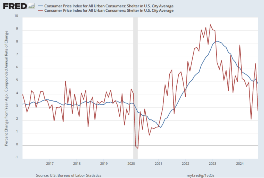
As the following figure shows, inflation in the price of shelter has been a significant contributor to headline inflation. The blue line shows 12-month inflation in shelter and the red line shows 1-month inflation in shelter. After rising in August, 12-month inflation in shelter resumed the decline that began in the spring of 2023, falling from 5.2 percent in August to 4.8 percent September. One-month inflation in shelter—which is much more volatile than 12-month inflation in shelter—declined sharply from 6.4 percent in August to 2.7 percent in September. The members of the FOMC are likely to find the decline in inflation in shelter reassuring as they consider another cut to the target for the federal funds rate at the committee’s next meeting on November 6-7. Shelter has a smaller weight of 15 percent in the PCE price index that the Fed uses to gauge whether it is hitting its 2 percent inflation target in contrast with the 33 percent weight that shelter has in the CPI.
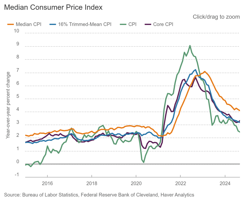
Finally, in order to get a better estimate of the underlying trend in inflation, some economists look at median inflation and trimmed mean inflation. Median inflation is calculated by economists at the Federal Reserve Bank of Cleveland and Ohio State University. If we listed the inflation rate in each individual good or service in the CPI, median inflation is the inflation rate of the good or service that is in the middle of the list—that is, the inflation rate in the price of the good or service that has an equal number of higher and lower inflation rates. Trimmed mean inflation drops the 8 percent of good and services with the higherst inflation rates and the 8 percent of goods and services with the lowest inflation rates.
As the following figure (from the Federal Reserve Bank of Cleveland) shows, median inflation (the orange line) declined slightly from 4.2 percent in August to 4.1 percent in September. Trimmed mean inflation (the blue line) was unchanged at 3.2 percent. These data provide confirmation that core CPI inflation at this point is likely running at least slightly higher than a rate that would be consistent with the Fed achieving its inflation target.
The FOMC cut its target for the federal funds rate by 0.50 percentage point (50 basis points) from 5.50 percent to 5.25 percent to 5.00 percent to 4.75 percent at its last meeting on September 17-18. Some economists and investors believed that the FOMC might cut its target by another 50 basis points at its next meeting on November 6-7. This inflation report makes that outcome less likely. In addition, the release of the minutes from the September 17-18 meeting revealed that a significant number of committee members may have preferred a 25 basis point cut rather than a 50 basis point cut at that meeting:
“However, noting that inflation was still somewhat elevated while economic growth remained solid and unemployment remained low, some participants observed that they would have preferred a 25 basis point reduction of the target range at this meeting, and a few others indicated that they could have supported such a decision.”
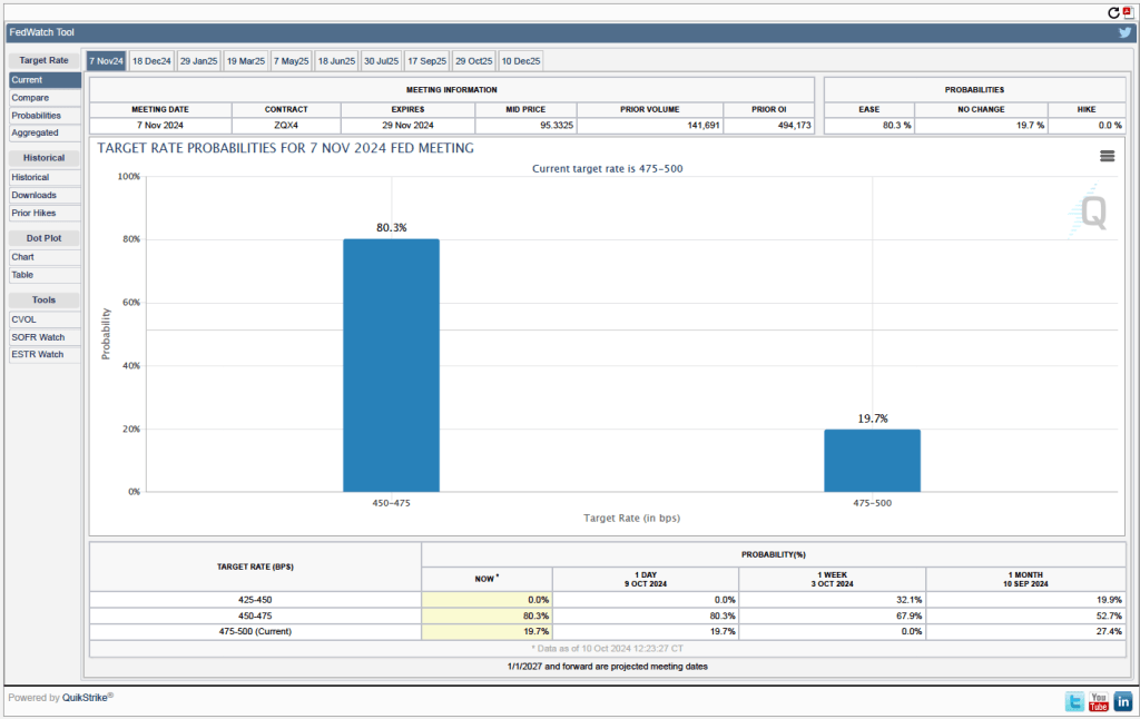
Investors who buy and sell federal funds futures contracts expect that the FOMC will cut its target for the federal funds rate by 0.25 percentage point at its November meeting. (We discuss the futures market for federal funds in this blog post.) As shown in the following figure, today these investors assign a probability of 80.3 percent to the FOMC cutting its target for the federal funds rate by 0.25 percentage point and a probability of 19.7 percent to the committee leaving its target unchanged.
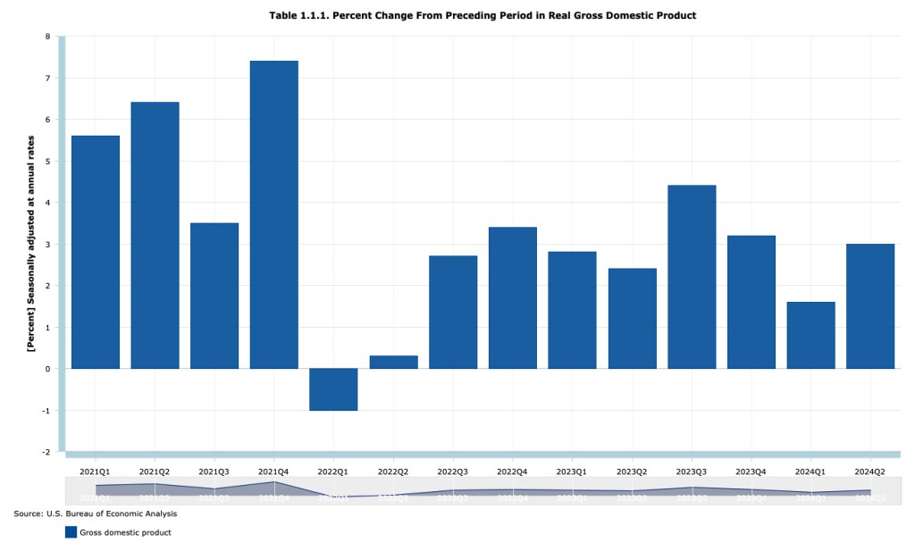
About one month after a calendar quarter ends, the Bureau of Economic Analyis (BEA) releases its advanced estimate of real GDP. In July 2022, the BEA’s advance estimates indicated that real GDP had declined in both the first and second quarters. A common definition of a recession is two consecutive quarters of declining real GDP. Accordingly, in mid-2022 there were a number of articles in the media suggesting that the U.S. economy was in a recession.
But, as we discussed at the time in this blog post, most economists don’t follow the popular definition of a recession as being two consecutive quarters of declining real GDP. Instead, as we discuss in Macroeconomics, Chapter 10, Section 10.3 (Economics, Chapter 20, Section 20.3), economists typically follow the definition of a recession used by the National Bureau of Economic Research (NBER): “A recession is a significant decline in activity spread across the economy, lasting more than a few months, visible in industrial production, employment, real income, and wholesale-retail trade.”
During the first half of 2022, the other data that the NBER tracks were all expanding rather than contracting. So, it seemed safe to conclude that despite the declines in real GDP in those quarters, the U.S. economy was not, in fact, in a recession.
That conclusion was confirmed by the BEA in September 2024 when it released its most recent revisions of real GDP . As the following table shows, although the BEA still estimates that real GDP fell during the first quarter of 2022, it now estimates that it increased during the second quarter.
In the earlier post from 2022, we also noted that the BEA publishes data on gross domestic income (GDI), as well as on GDP. As we discuss in Chapter 8, Section 8.1, when considering the circular-flow diagram, the value of every final good and service produced in the economy (GDP) should equal the value of all the income in the economy resulting from that production (GDI). The BEA has designed the two measures to be identical by including in GDI some non-income items, such as sales taxes and depreciation. But as we discuss in the Apply the Concept, “Should We Pay More Attention to Gross Domestic Income?” GDP and GDI are compiled by the BEA from different data sources and can sometimes significantly diverge.
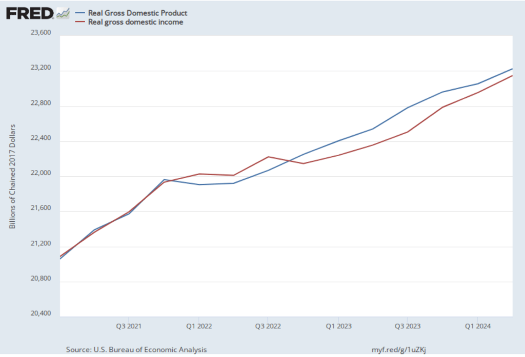
We noted that although, according to the BEA’s advance estimates, real GDP declined during the first two quarters of 2022, real GDI increased. The following figure shows movements in real GDP and real GDI using the current estimates from the BEA. The revised estimates now show real GDP falling the first quarter of 2021 and increasing in the second quarter while real GDI is still estimated as rising in both quarters. The revisions closed some of the gap between real GDP and real GDI during this period by increasing the estimate for real GDP, which indicates that the advance estimate of real GDI was giving a more accurate measure of what was happening in the U.S. economy.
The figure shows that the revised estimates indicate that real GDP and real GDI moved closely together during 2021, differed somewhat during 2022—with real GDI being greater than real GDP—and differed more substantially during 2023 and 2024—with real GDP now being greater than real GDI. Because the two measures should be the same, we can expect that further revisions by the BEA will bring the two measures closer together.
It’s even possible, but unlikely, that further revisions of the data for 2022 could again present us with the paradox of real GDP declining for two quarters despite other measures of economic activity expanding.
Supports: Macroeconomics, Microeconomics, Economics, and Essentials of Economics, Chapter 3, Section 3.1.
Photo from theathletic.com
Caitlin Clark had a sensational college career at the University of Iowa, being named National Player of the Year in her junior and senior years. She was chosen first by the Indiana Fever in the 2024 Women’s National Basketball Association (WNBA) draft of college players. Her popularity drew large crowds to both her home and away games during the 2024 season.
In 2023, the Indiana Fever sold an average of 4,067 tickets to its home games. In 2024, with Clark on the team, the Fever sold an average of 17,036 to its home games. The average price the Fever charged per ticket increased from $60 in 2023 to $110 in 2024. As an article on theathletic.com put it: “Despite the higher price point, even more tickets were sold [by the Fever] this year.”
Can we conclude from this information that Caitlin Clark is so popular that the demance curve for Fever tickets is upward sloping? Briefly explain.
Solving the Problem Step 1: Review the chapter material. This problem is about the effect of a price change on the quantity demand of a good or service, so you may want to review Chapter 3, Section 3.1, “The Demand Side of the Market.”
Step 2: Answer the question by explaining whether it’s likely that the demand curve for tickets to Fever games is upward sloping. It’s unlikely that the demand curve for tickets to Fever games is upward sloping. The law of demand states that, holding everything else constant, when the price of a product rises, the quantity demanded of the product will decrease. When the Fever raised ticket prices from $60 in 2023 to $100 in 2024, we would expect the result to be a movement up the demand curve for tickets, resulting in fewer tickets sold, provided that everything else that would affect the demand for tickets was constant between 2023 and 2024. But everything wasn’t constant because the Fever had Clark on the team in 2024 but not in 2023. Her popularity increased the demand for tickets, shifting the demand curve to the right. In other words, the shift in demand allowed the Fever to sell more tickets at a higher price—moving from a price of $60 and a quantity of 4,067 on the 2023 demand curve to a price of $110 and a quantity of 17,036 on the 2024 demand curve.
Glenn serves on the the Grand Bargain Committee, chaired by Michael Strain of the American Enterprise Institute and Isabel Sawhill of the Brookings Institution. The committee, whose members span the political spectrum, have prepared a report that addresses some of the country’s most pressing economic and social problems.
Glenn and Michael Strain prepared the following introduction to the report. Below there is a link to the whole report.
The views expressed in this report are those of the individual authors who collectively constitute the Grand Bargain Committee, co-chaired by Michael R. Strain and Isabel V. Sawhill. This report was sponsored by the Center for Collaborative Democracy and was prepared independent of influence from the center and from any other outside party or institution. It is being published by the Bipartisan Policy Center as an example of how people with diverse views and political leanings can find common ground. The recommendations are strictly those of the policy experts and do not necessarily reflect the views of any organization or those of the BPC. All data are current as of November 2023.
By: Eric Hanushek, G. William Hoagland, Douglas Holtz-Eakin, R. Glenn Hubbard, Maya MacGuineas, Richard V. Reeves, Robert D. Resichauer, Gerard Robinson, Isabel V. Sawhill, Diane Schanzenbach, Richard Schmalensee, Michael R. Strain, and C. Eugene Steuerle.
Introduction
The United States faces serious economic and social challenges, including:
The underlying economic growth rate has slowed, as have opportunities for people to move up the economic ladder.
Our education system fails too many children and leaves many more with fewer opportunities than they deserve.
The nation is not rising to the challenge of addressing climate change.
Both our health care system and the health of our population need improvement.
Our income tax system is broken, generating tax revenue in an inefficient and unfair manner.
And the national debt is growing at an unsustainable pace, threatening long-term economic growth, crowding out needed investments in economic opportunity, and placing the nation’s ability to respond to a future crisis at risk.
To address these problems, the Center for Collaborative Democracy commissioned subject matter experts—progressives, centrists, and conservatives—to develop a “Grand Bargain” encompassing all six issues. The policy debate typically puts these problems into silos, and within each silo, powerful forces support the status quo. This report seeks to break down these silos. Dealing with them all at once—in a Grand Bargain—is a more promising strategy than dealing with them individually, because it allows for different parties to strike deals across policy issues, not just within a single issue.
For example, implementing a carbon tax to address climate change seems impossibly difficult. So does increasing accountability for teacher performance. Trading one for the other might be easier than pursuing both in isolation. Fixing the structural budget deficit by reducing entitlement spending is an enormous political challenge. So is increasing spending on programs that advance economic opportunity. Doing both at the same time could be more politically feasible than addressing them separately.
In this context, the group of experts met for several months in 2023 to share perspectives and ideas and to come up with sensible policies in each of these areas: economic growth and mobility; education; environment; health; taxes; and the federal budget. The end result is this report, which is being published by the Bipartisan Policy Center as an example of how people with diverse views and political leanings can find common ground.
This report is short, consisting of less than 30 pages of text. Its brevity is by design. This constraint forced the group to stay focused on issues and recommendations that matter the most. The focus of the report is on concepts. It is designed to answer such questions as, “How should the nation’s approach to education or to the federal budget change? What fundamental reforms are required to increase the underlying rates of economic growth and upward mobility?” Focusing on concepts means not focusing on policy details, including the details of implementing our recommendations and of transitioning across policy regimes. Our lack of attention to policy details does not mean we do not recognize their importance. Of course, we do, and many members of the group have spent much of their careers studying and designing public policies. Instead, we focus on concepts because we believe the United States needs to return to a discussion of first principles. This report advances that objective.
Not every member of the group agrees with every recommendation in this report. That is not surprising given the diversity of views in the group, and the difficulty and complexity of many of the issues we address. Despite this disagreement, we were able to have an informed and constructive discussion about these economic issues, to find compromises, and to come up with a set of recommendations that we believe, on balance, would greatly strengthen the country and improve people’s lives.
We believe in the importance of a market economy. Free markets have led to unprecedented growth and innovation, along with rising incomes, over the past three centuries. But government also has a role to play. To unleash more growth, we need to curtail unneeded or overly costly regulations and to create a tax system that encourages investment spending and innovation. To bring prosperity to more people, we need policies that will enable more people to benefit from economic growth through investment in their education and skills. For this reason, we put a great deal of emphasis on improving education for children, on training or retraining for adult workers, and on subsidizing the earnings of low-wage workers when necessary while maintaining a safety net for those who cannot work.
Our proposals are designed to advance certain underlying values and themes: Work and savings should be rewarded, investment should be encouraged over consumption, public assistance should be better targeted to those most in need, the tax system should be more progressive, and the nation should invest relatively more in the young and spend relatively less on the elderly.
Our specific proposals in each area are as follows:
On economic growth and mobility, we recommend investing in the education and training of workers, through community colleges and apprenticeships. We call for a more skill-based immigration system and for more immigrants; for encouraging innovation by investing more in basic research; for reducing taxes on new investment; for curbing unneeded regulation; for reducing the national debt; and for encouraging participation in economic life by increasing the generosity of earnings subsidies for low-wage workers.
On education, we recommend improving the teacher workforce at the K-12 level; paying teachers more but strengthening the link between pay and performance; maintaining educational standards and accountability while narrowing gaps by race and class; expanding school choice; and recognizing the role that parents and families must play in students’ learning.
On the environment, our main recommendation is to adopt a carbon tax. We also call for reducing methane emissions; expanding federal authority in the planning, siting, and permitting of the national electric transmission system; and repealing the renewable fuel standard that requires refiners to blend corn ethanol into the fuel they sell.
On health, we call for giving more attention to the social determinants of poor health with a focus on the need for better nutrition, for rationalizing existing subsidies for health care, and for reducing health care costs.
On taxes, we call for increasing tax revenue as a share of annual gross domestic product (GDP), and for that revenue to be raised in a manner that is more progressive, efficient, and simple than under current law, while also increasing the incentive to save and invest. For the business sector, that means allowing the expensing of investment expenditures and moving toward equal treatment of the corporate and noncorporate sectors.
On the federal budget, we recommend putting the debt as a share of annual GDP on a sustainable trajectory with a comprehensive package of reforms made up of a rough balance between tax increases and spending cuts in the initial years, phasing into a much larger share of the savings coming from spending cuts over time.
Most of these recommendations are at the federal level, but some are at the state and local level, particularly our education recommendations.
In the spirit of a Grand Bargain, these recommendations advance common goals and values through compromises both within and across policy areas. For example, one of our values is reflected in the goal of refocusing government spending on those who truly need it, and another is to restore fiscal responsibility. To accomplish this, we call for slower growth in Social Security and Medicare benefits for affluent seniors to reduce the major driver of the national debt, but we also protect vulnerable seniors and spend more on the education of children and on earnings subsidies for the working poor. We recommend adopting a carbon tax because it will simultaneously advance our goals of supporting the environment, increasing tax revenue, and boosting dynamism by encouraging innovation in the energy sector.
We believe the analysis and recommendations in this report point a path forward for the nation, but we offer them in a spirit of humility, understanding that others will disagree. We hope that this report catalyzes a much needed debate about the future of our nation.
Image generated by GTP-4o of “an apartment building in Amersterdam.”
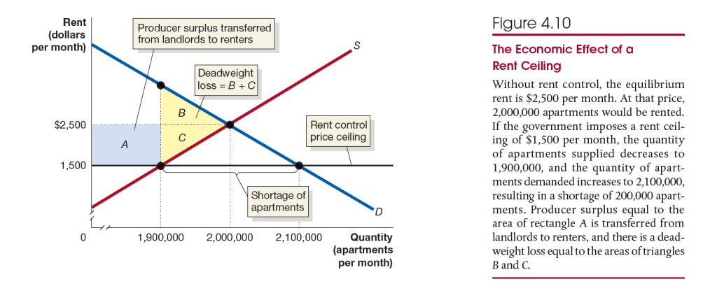
Recent articles in the media discussed the effects of rent control on the market for apartments in the Netherlands and in Stockholm, the capital of Sweden. The articles describe a situation that is consistent with the analysis in Chapter 4, Section 4.3. Figure 4.10 shows the expected results from the imposition of a rent control law. Some renters gain by living in apartments at below the equilibirum market rent, but the shortage of apartments resulting from the price ceiling means that some renters are unable to find apartments. As with other price controls, rent ceilings impose a deadweight loss on the economy, shown in the figure as the areas B + C.
An article on bloomberg.com discusses the effect on the market for apartments in the Netherlands of the passage in June of the Affordable Rent Act. The act raised the fraction of apartments covered by rent control from about 80 percent to 96 percent. The expansion of rent control appears to have led to an increased shortage of apartments. The article quotes one teacher who has been unable to find an apartment for her family as saying: “The cost isn’t the problem, but a real shortage of housing is.”
The article indicates that some landlords who doubt they can earn a profit under the new law are selling their buildings. If the buildings are converted to other uses, the shortage of apartments will be increased. The article mentions another unintended change to the apartment market from the provision of the new law that requires leases to be open-ended. Some landlords fear that as a result they may find themselves unable to evict tenants, however troublesome the tenants may be. In response, these landlords are giving priority to foreigners, who they believe are likely to move more often.
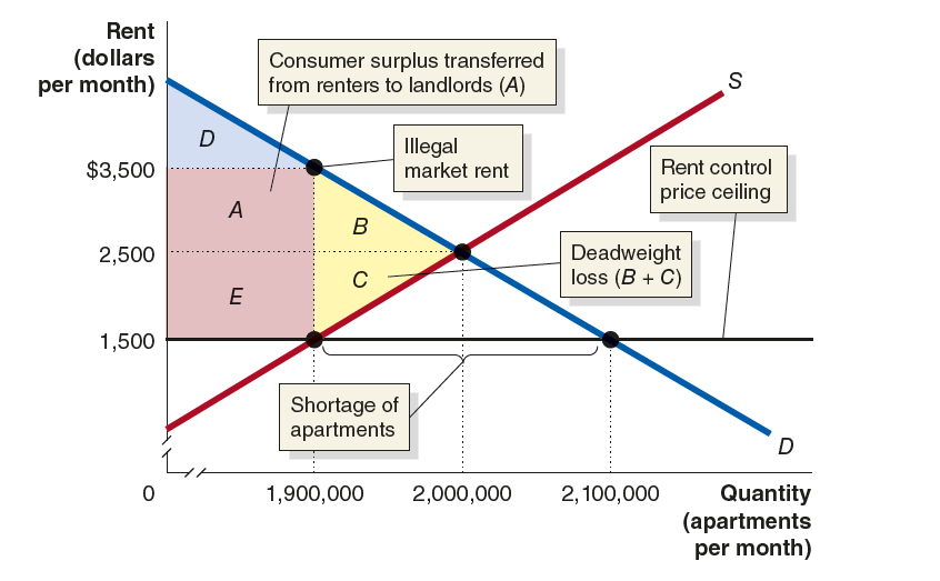
An article in the Economist looks at another aspect of rent control. The following figure is reproduced from Solved Problem 4.3. It shows that because rent control leads to a shortage of apartments it creates an incentive for tenants and landlords to agree to a rent that is higher than the legal rent ceiling. In this example, renters who are unable to find an apartment at the rent control ceiling of $1,500 may bid up the rent to $3,500—which in this example is $1,000 higher than the market equilibrium rent in the absence of rent control—rather than not be able to rent an apartment. Clearly, renters paying this illegal rent are worse off than they would be if there were no rent control law.
According to the article in the Economist, the average time on a waiting list for a rent controlled apartment is 20 years. Not surprisingly, “Young Swedes often have to put up with expensive sublets agreed to under the table,” for which they typically pay rents above both the rent control ceiling and the market equilibrium rent. Most economists agree that expanding the quantity of available housing by making it easier to build homes and apartments is a better way of reducing housing costs than is imposing rent controls.
President Lyndon Johnson signing the Economic Opportunity Act in 1964. (Photo from Wikipedia)
In 1964, President Lyndon Johnson announced that the federal government would launch a “War on Povery.” In 1988, President Ronald Regan remarked that “some years ago, the Federal Government declared war on poverty, and poverty won.” Regan was exaggerating because, however you measure poverty, it has declined substantially since 1964, although the official poverty rate has remained stubbornly high since the early 1970s.
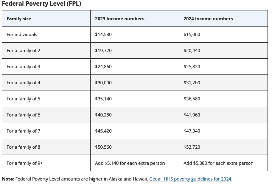
Each year the U.S. Census Bureau calculates the official poverty rate—the fraction of the population with incomes below the federal poverty level, often called the poverty line. The following table shows the poverty line for the years 2023 and 2024 illustrating how it varies with the size of a household:
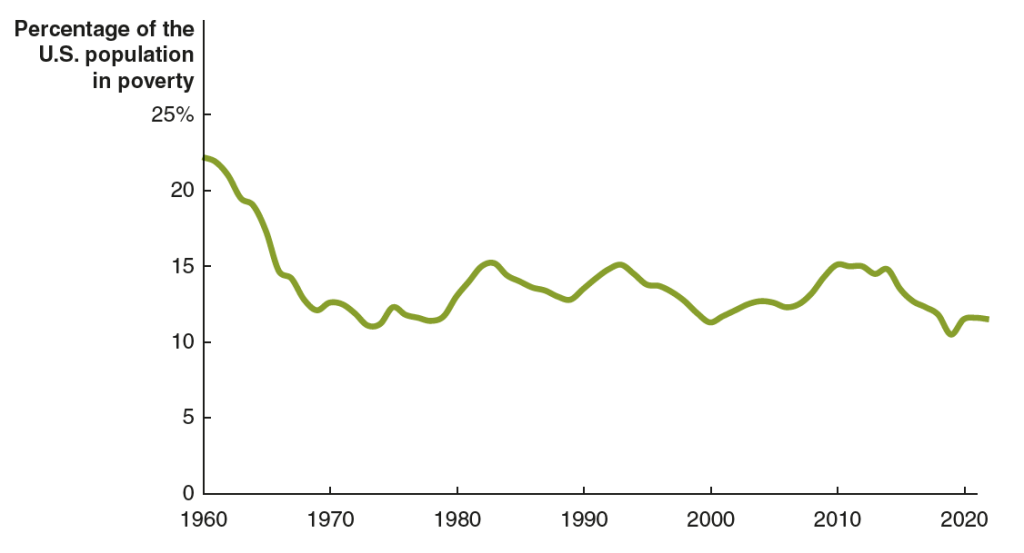
The following figure shows the official poverty rate for the years from 1960 to 2022. The poverty rate in 1960 was 22.2 percent. By 1973, it had been cut in half to 11.1 percent. The decline in the poverty rate largely stopped at that point. In the following years the official poverty rate fluctuated but stopped trending down. In 2022, the poverty rate was 11.5 percent—actually higher than in 1973. (The Census Bureau will release the poverty rate for 2023 later this month.)
But is the official poverty rate the best way to measure poverty? In Microeconomics, Chapter 17, Section 17.4 (Economics, Chapter 27, Section 27.4), we discuss some of the issues involved in measuring poverty. One key issue is how income should be measured for purposes of calculating the poverty rate. In an academic paper, Richard Burkhauser, of the University of Texas, Kevin Corinth, of the American Enterprise Institute, James Elwell, of the Congressional Joint Committee on Taxastion, and Jeff Larimore, of the Federal Reserve Board, carefully consider this issue. (The paper can be found here, although you may need a subscription or access through your library.)
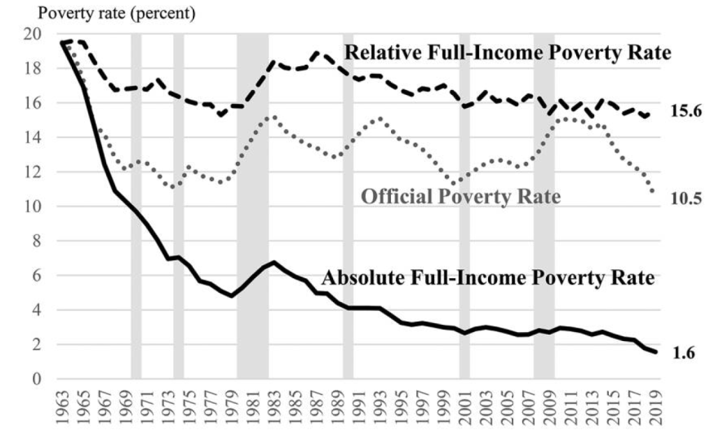
They find that using an adjusted measure of the poverty line and a fuller measure of income results in the poverty rate falling from 19.5 percent in 1963 to 1.9 percent in 2019. In other words, rather than the poverty rate stagnating at around 11 percent—as indicated using the official poverty numbers—it actually fell dramatically. Rather than progress in the War on Poverty having stopped in the early 1970s, these results indicate that the war has largely been won. The authors, though, provide some important qualifications to this conclusion, including the fact that even 1.9 percent of the population represents millions of people.
Discussions of poverty distinguish between absolute poverty—the ability of a person or family to buy essential goods and services—and relative poverty—the ability to buy goods and services similar to those that can be purchased by individuals and families with the median income. The authors of this study argue that in launching the War on Povery, President Johnson intended to combat absolute poverty. Therefore, the authors start with the poverty line as it was in 1963 and increase the line each year by the rate of inflation, as measured by changes in the personal consumption expenditures (PCE) price index.
To calculate what they call “the absolute full-income poverty measure (FPM)” they include in income both cash income and “in-kind programs designed to fight poverty, including food stamps (now the Supplemental Nutrition Assistance Program [SNAP]), the schoollunch program, housing assistance, and health insurance.” As noted earlier, using this new definition, the overall poverty rate declined from 19.5 percent in 1963 to 1.9 percent in 2019. The Black poverty rate declined from 50.8 percent in 1963 to 2.9 percent in 2019.
The author’s find that the War on Poverty has been less successful in reducing relative poverty. Linking increases in the poverty line to increases in median income results in the poverty rate having decreased only from 19.5 percent in 1963 to 15.6 percent in 2019. The authors also note that not as much progress has been made in fulfilling President Johnson’s intention that: “The War on Poverty is not a struggle simply to support people, to make them dependent on the generosity of others.” They find that the fraction of working-age people who receive less than half their income from working has increased from 4.7 percent in 1967 to 11.0 percent in 2019.
The following figure from the authors’ paper shows the offical poverty rate, the absolute full-income poverty rate—which the authors believe does the best job of representing President Johnson’s intentions when he launched the War on Poverty—and the relative poverty rate.
Because of disagreements on how to define poverty and because of the difficulty of constructing comprehensive measures of income—difficulties that the authors discuss at length in the paper—this paper won’t be the last word in assessing the results of the War on Poverty. But the paper provides an important new discussion of the issues involved in measuring poverty.