Image generated by GTP-4o of a woman singer performing at a concert.
The answer to the question in the title is “yes” according to a column by James Mackintosh in the Wall Street Journal. In the Apply the Concept “Taylor Swift Tries to Please Fans and Make Money,” in Chapter 11 of Microeconomics, we discussed how for her The Eras Tour, Taylor Swift reserved more than half of the concert tickets for her “verified fans.” The tickets sold to verified fans for an average price of $250.
On the resale market, prices of the tickets soared to $1,000 or more. Yet only about 5 percent of tickets purchased by verified fans were resold. Mackintosh’s wife and “eldest offspring” were in in the other 95 percent—they had purchased their tickets at a low price but wouldn’t resell them at a much higher price. Moreover—and this is where Mackintosh sees economics as breaking—if they didn’t already have the tickets they wouldn’t have bought them at the current high price.
Not being willing to buy something at a price you wouldn’t sell it for is inconsistent behavior because it ignores a nonmonetary opportunity cost. (As we discuss in Chapter 10, Section 10.4.) If Mackintosh’s wife won’t sell her ticket for $1,000, she incurs a $1,000 opportunity cost, which is the amount she gives up by not selling the ticket. The two alternatives—either paying $1,000 for a ticket or not receiving $1,000 by declining to sell a ticket—amount to exactly the same thing.
Mackintosh recognizes that the actions of his wife and offspring reflect what he calls a “mental bias,” which he correctly labels the endowment effect: The tendency to be unwilling to sell something you already own even if you are offered a price greater than the price you would be willing to buy the thing for if you didn’t already own it.
As we discuss in Chapter 10, the endowment effect is one of a number of results from behavioral economics, which is the study of situations in which people make choices that don’t appear to be economically rational. So, Mackintosh’s family—and other Swifties—didn’t break economics. Instead, they demonstrated one of the results of behavioral economics.
Photo of Federal Reserve Chair Jerome Powell from federalreserve.gov
Federal Reserve chairs often take the opportunity of the Kansas City Fed’s annual monetary policy symposium held in Jackson Hole, Wyoming to provide a summary of their views on monetary policy and on the state of the economy. In speeches, Fed chairs are careful not to preempt decisions of the Federal Open Market Committee (FOMC) by stating that policy changes will occur that the committee hasn’t yet agreed to. In his speech at Jackson Hole on Friday (August 23), Powell came about as close as Fed chairs ever do to announcing a policy change in a speech.
In the speech, Powell indicated that: “The time has come for policy to adjust. The direction of travel is clear, and the timing and pace of rate cuts will depend on incoming data, the evolving outlook, and the balance of risks.” The statement is effectively an announcement that the FOMC will reduce its target for the federal funds rate at its next meeting on September 17-18. By referring to “the timing and pace of rate cuts,” Powell was indicating that the FOMC was likely to eventually reduce its target for the federal funds rate well below its current 5.25 percent to 5.50 percent, although the reductions will be spread out over a number of meetings.
The minutes of the FOMC’s last meeting on July 30-31 were released on August 21. The minutes stated that: “The vast majority [of committee members] observed that, if the data continued to come in about as expected, it would likely be appropriate to ease policy at the next meeting.” The apparent consensus at the July meeting that the target for the federal funds rate should be reduced at the September meeting was likely the key reason why Powell was so forthright in his speech.
In his speech, Powell summarized his views on the reasons that inflation accelerated in 2021 and why it has slowly declined since reaching a peak in the summer of 2022:
“[The analysis of events that Powell supports] attributes much of the increase in inflation to an extraordinary collision between overheated and temporarily distorted demand and constrained supply. While researchers differ in their approaches and, to some extent, in their conclusions, a consensus seems to be emerging, which I see as attributing most of the rise in inflation to this collision. All told, the healing from pandemic distortions, our efforts to moderate aggregate demand, and the anchoring of expectations have worked together to put inflation on what increasingly appears to be a sustainable path to our 2 percent objective.”
As he has over the past three years, Powell emphasized the importance of expectations having remained “anchored,” meaning that households and firms continued to expect that the annual inflation rate would return to 2 percent, even when the current inflation rose far above that rate. We discuss how expectations of inflation affect the current inflation rate in Macroeconomics, Chapter 17 (Economics, Chapter 27).
Image of servers in a restaurant generated by ChatGTP-4o.
How should you track over time the real wagees of low-wage workers? If you are interested in income mobility, you would want to track the experience over the course of their working lives of individuals who began their careers in low-wage occupations. Doing so would allow you to measure how well (or poorly) the U.S. economy succeeds in providing individuals with opportunities to improve their incomes over time.
You might also be interested in how the real wages of people who earn low wages has changed over time. In this case, rather than tracing the wages over time of individuals who earn low wages when they first enter the labor market, you would look at the real wages of people who earn low wages at any given time. The simplest way to do that analysis would be using data on the average nominal wage earned by, say, the lowest 20 percent of wage earners, and deflate the average nominal wage by a price index to determine the average real wage of these workers. How the average real wage of low-wage workers varies over time provides some insight into the changing standard of living of low-wage workers.
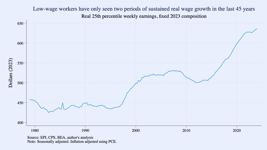
In a recent Substack post, Ernie Tedeschi, Director of Economics at the Budget Lab research center at Yale University, has carried out a careful analysis of movements over time in the average real wage of low-wage workers. Tedeschi points out a complicating factor in this analysis: “The population has gotten older over time and more educated. The workforce looks different too, with more workers in services and fewer in manufacturing. Shifting populations means that comparisons of workers aren’t apples-to-apples over time.”
To correct for these confounding factors, Tedeschi constructs a low-wage index that makes it possible to examine the real wage of low-wage workers, holding constant the composition of low-wage workers with respect to “sex, age, race, college education, and broad industry and occupation” at the values of these characteristics in 2023. Using this approach, makes it possible to separate changes in wages of workers with given characteristics from changes in wages that occur because the average characteristics of workers has changed. For example, on average, workers who are older or who have more years of education will be more productive and, therefore, on average will earn higher wages than will workers who are younger or have fewer years of education.
The following figure from Tedeschi’sSubstack post shows movements in his low-wage index during each quarter from the first quarter of 1979 to the first quarter of 2024, with “low wage” defined as workers at the 25th precentile of the distribution of wages. (That is, 24 percent of workers receive lower wages and 75 percent of workers receive higher wages than do these workers.) The index shows that a low-wage worker in 2024 has a much higher real wage than a low-wage worker in 1979, but the increase in the average real wage occurs mainly during two periods: 1997–2007 and 2014–2024. (Tedeschi uses the person consumption expenditures (PCE) price index to convert nominal wages to real wages.)
A more complete discussion of Tedeschi’s methods and results can be found in his blog post.
Supports: Microeconomics and Economics, Chapter 6, and Essentials of Economics, Chapter 7.
Photo from the New York Times.
An article in the Wall Street Journal reported that Starbucks during certain periods is cutting by 50 percent the prices of many of its coffees, including its Frappuccino. The article also noted that: “Many restaurant chains are pumping out new deals this year in a bid to reverse weak traffic.” The article also quoted a Starbucks spokesman as saying that Starbucks is cutting prices “to ensure that consumers who are facing a challenging economic environment continue to visit its cafes.”
What is Starbucks likely assuming about the price elasticity of demand for Frappuccinos?
Suppose that after cutting its price of Frappuccinos by 50 percent, the quantity of Frappuccinos sold increases by 20 percent. Ignoring any information other than the values of the price cut and the quantity increase, calculate the price elasticity of demand for Frappuccinos. Considering only the value of the price elasticity of demand you calculated, will Starbucks earn more revenue or less revenue from selling Frappuccions as a result of the price cut? Briefly explain.
Suppose that during the time that Starbucks cuts the price of Frappuccinos, competing coffee houses also cut the prices of their coffees. How will this fact affect your answer to part b.? Briefly explain.
Does the fact that, because of inflation, some consumers are facing a “challenging economic environment” affect your answer to part b.? Briefly explain.
Solving the Problem
Step 1: Review the chapter material. This problem is about the determinants of the price elasticity of demand and the effect of the value of the price elasticity of demand on a firm’s revenue following a price change, so you may want to review Chapter 6, Section 6.2 and Section 6.3.
Step 2: Answer part a. by explaining what Starbucks is likely assuming about the price elasticity of demand for Frappuccinos. Starbucks appears to be assuming that the demand for Frappuccions is price elastic, in which case a cut in the price will result in a more than proportional increase in the quantity of Frappuccions demanded.
Step 3: Answer part b. by using the values given to calculate the price elasticity of demand for Frappuccions and explain whether as a result of the price cut Starbucks will earn more or less revenue from selling Frappuccinos.If all other factors affecting the demand for a product are held constant, the price elasticity of demand equals the percentage change in the quantity demanded divided by the percentage change in price. Therefore, in this case the price elasticity of demand for Frappuccinos equals 20%/–50% = –0.4. Therefore, relying just on the information on the changes in the price and quantity demanded, the demand for Frappuccinos is price inelastic. As explained in Section 6.5, when demand is price inelastic, a cut in price will result in a decrease in revenue.
Step 4: Answer part c. by explaining whether other coffee houses cutting the prices of their coffees will affect your calculation from part b. of the price elasticity of demand for Frappuccinos. The calculation in part b. assumes that during the time that Starbucks cuts the price of Frappuccinos, nothing else that affects demand will have changed. We know that the coffees sold by other coffee houses are substitutes for Frappuccinos. So we would expect that if other coffeehouses cut the prices of their coffees, the demand curve for Frappuccinos will shift to the left. The 20 percent increase in the quantity of Frappuccions sold reflects the effects of both the price cut and the shift in the demand curve for Frappuccinos. Therefore our calculation of the price elasticity of demand for Frappuccinos is inaccurate. It’s likely that the price elasticity is larger (in absolute value) than the value we caculated in part b.
Step 5: Answer part d. by explaining whether the fact that some consumers are facing a “challenging economic environment” affects your answer to part b. The answer to part d. is similar to the answer to part c. If the fact that some consumers are facing a “challenging economic environment” means that these consumers are less likely to be buying coffee and other products away from home, then the demand curve for Frappuccinos will have shifted to the left during the period that Starbucks cut the price of these coffees. As a result, the value we computed for the price elasticity of demand in part b. will be inaccurate. Taken together, the factors mentioned in parts c. and d. indicate the difficulties that firms have in calculating the price elasticity of demand for their products during a time period when several factors that affect the demand for the products may be changing.
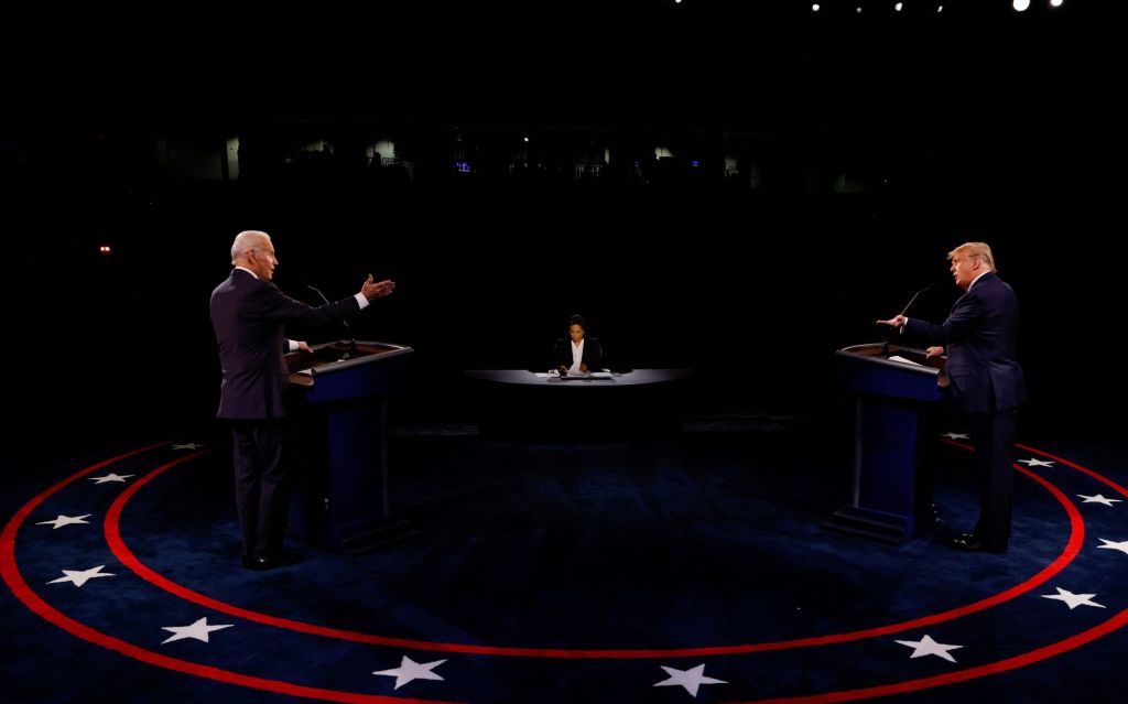
Presidents Biden and Trump during one of their 2020 debates. (Photo from the Wall Street Journal)
On the eve of first debate between President Joe Biden and former President Donald Trump, Glenn reflects on the fundamentals of sound economic policy. This essay first appeared inNational Affairs.
The advent of “Bidenomics” has resurrected decades-old debates about the merits of markets versus industrial policy. When President Joe Biden announced his eponymous strategy in June 2023, he blasted what he described as “40 years of Republican trickle-down economics” and insisted that he would seek instead to build “an economy from the middle out and the bottom up, not the top down.” He would achieve this through “targeted investments” in technologies like semiconductors, batteries, and electric cars — all of which featured heavily in initiatives like the CHIPS and Science Act and the Inflation Reduction Act. Yet despite the president’s professed support for a “middle out” economics, Bidenomics has thus far proven to be less of an intellectual framework than a set of well-intended yet ill-fated industrial-policy interventions implemented from the top down.
Some conservatives have joined Biden in embracing industrial policy. Writing recently in these pages, Republican senator Marco Rubio of Florida asserted that while it is difficult to “get industrial policy right, conservatives can and must take ownership of this space to keep the American economy strong and free.” Former president Donald Trump, for his part, staunchly advocates heavy tariffs to promote domestic manufacturing.
Conservatives who adopt their own version of protectionist tinkering with markets are missing an important opportunity. As mercantilism’s decline did for classical liberalism in the 19th century and Keynesianism’s misadventures did for neoliberalism in the 20th, Bidenomics’ failures offer an opening for the right to champion a new type of economics — one that puts opportunity for the people ahead of the economic rules of the game.
Rapid globalization and technological change have left too many Americans behind. But the answer is not for the state to invest in costly projects with dubious prospects, nor is it to adopt a strictly laissez-faire approach to the economy. By reviving classically liberal ideas about competition and opportunity in the face of change, conservatives can promote an alternative economics that retains the enormous benefits of markets and openness while putting people first.
LIBERALISM’S RISE AND FALL
Before “Bidenomics” became a popular term, national-security advisor Jake Sullivan hinted at the president’s economic priorities in an April 2023 speech at the Brookings Institution. There, he declared that a “new Washington consensus” had formed around a “modern industrial and innovation strategy,” which would correct for the excesses of the free-market orthodoxy propagated by the likes of Adam Smith, Friedrich Hayek, and Milton Friedman.
This orthodoxy, according to Sullivan, “championed tax cutting and deregulation, privatization over public action, and trade liberalization as an end in itself,” all of which eroded the nation’s industrial and social foundations. Finally, after nearly three decades of such policies, two “shocks” — the global financial crisis of 2007-2009 and the Covid-19 pandemic — ”laid bare the limits” of liberalism. The time had come, Sullivan concluded, to dispense with decades of policies touting the benefits of markets and free trade — and economists would just have to get over it.
The Biden administration’s assault on open markets and free trade is odd in some respects. Scholars at the Peterson Institute for International Economics — located just across the street from Brookings — concluded in a 2022 report that, thanks to America’s openness to globalization, trillions of dollars in economic benefits have flowed to U.S. households. Moreover, the United Nations estimates that integrating China, India, and other economies into the world trading order has brought one billion individuals out of poverty since the 1980s. The impact of technological change as a driver of growth and incomes is larger still. Juxtaposing such outcomes with the administration’s grievances calls to mind the popular outcry in Monty Python’s Life of Brian: “What have the Romans ever done for us?” Quite a lot, in fact.
Proponents of free markets have clashed with advocates of government intervention before, most notably at the dawn of classical liberalism toward the end of the 18th century and the advent of neoliberalism during the first half of the 20th. These contests were not so much battles of ideas as they were intellectual critiques of real-life policy failures.
In 1776, Adam Smith’s Inquiry into the Nature and Causes of the Wealth of Nations threw down the gauntlet. The book was radical, offering a sharp rebuke of the economic-policy order of the day. Mercantilism — or the “mercantile system,” as Smith called it — assumed that the world’s wealth is fixed, and that a state wishing to improve its relative financial strength would have to do so at the expense of others by maintaining a favorable balance of trade — typically by restricting imports while encouraging exports. Recognizing merchants’ role in generating domestic wealth, mercantilist states also developed government-controlled monopolies that they protected from domestic and foreign competition through regulations, subsidies, and even military force.
Predictably, this system enriched the merchant class. But it did so at the expense of the poor, who were subject to trade restrictions and import taxes that drove up the price of goods. It also stunted business growth, expanded the slave trade, and triggered inflation in regions with little gold and silver bullion on hand.
Smith turned the mercantilist view on its head, insisting that the real touchstone of “the wealth of a nation” was not the amount of gold and silver held in its treasury, but the value of the goods and services it produced for its citizens to consume. To maximize a nation’s wealth, he argued that the state should unleash its population’s productive capacity by liberating markets and trade. Setting markets free, he observed, would enable firms to specialize in generating the goods they produced most efficiently, and to exchange surpluses of those goods for specialized goods produced by others. This approach would spread the benefits of free trade throughout the population.
While sometimes caricatured as a full-throated endorsement of laissez-faire economics, Wealth of Nations also recognized that government played an important role in sustaining an environment that would allow free markets to flourish. This included protecting property rights, building and maintaining infrastructure, upholding law and order, promoting education, providing for national security, and ensuring competition among firms. Smith cautioned, however, that government officials should be careful not to distort markets unnecessarily through such mechanisms as taxation and overregulation, and should avoid accumulating large public debts that would drain capital from future productive activities.
Mercantilism did not suddenly fall away after Smith’s critique; it continued to dominate much of the world’s economic order for another half-century. But eventually, Smith’s arguments in favor of market liberalization carried the day. For much of the 19th and early 20th centuries, free markets and free trade facilitated unprecedented prosperity in the West.
A parallel series of events occurred during the 1930s and ’40s, when Friedrich Hayek and John Maynard Keynes famously (and nastily) debated economic theory in the pages of the Economic Journal. That contest, too, revolved around what was happening on the ground: the Great Depression and increasing government investment in industry. Keynes contended that market economies experience booms and busts based on fluctuations in aggregate demand, and that the government could mitigate the harms of recessions by stimulating that demand through increased spending. Hayek disagreed, arguing that such large-scale public spending programs as those Keynes proposed would prompt not just market inefficiency and inflation, but tyranny.
During the 1950s and ’60s, Milton Friedman took on Keynes’s theories, asserting instead that the key to stimulating and maintaining economic growth was to control the money supply. He also expanded on Hayek’s case for free markets as necessary elements of free societies: As he wrote in Capitalism and Freedom, economic freedom serves as both “a component of freedom broadly understood” and “an indispensable means toward the achievement of political freedom.”
Of course Hayek and Friedman, like Smith before them, did not immediately win the debate; Keynesianism dominated America’s economic policy for decades after the Second World War. But by the mid-1970s, rising inflation and slowed economic growth pressured policymakers to consider a different approach. Hayek and Friedman’s arguments — now often referred to collectively as “neoliberalism” — ultimately won over important political figures like Ronald Reagan and Bill Clinton in the United States and Margaret Thatcher and Tony Blair in Britain. It had a major impact on each of their economic-policy initiatives, which typically combined tax cuts and deregulation with reduced government spending and liberalized international trade.
The upshot of that liberal market order is reflected in the 2022 findings of the Peterson Institute outlined above — namely the trillions of dollars in economic benefits that have flowed to American households. In a similar vein, the institute found in a 2017 report that between 1950 and 2016, trade liberalization combined with cheaper transportation and communication owing to technological change increased per-household GDP in the United States by about $18,000. The benefits of economic liberalism have thus been and continue to be massive.
NEOLIBERAL OVERCORRECTION
For all the prosperity it brought to the world, market-induced change in an era of globalization and rapid technological advance also entailed significant costs. Leaders across the political spectrum celebrated the former but paid little attention to the latter, which hit low- and medium-skilled American workers particularly hard. As global competition intensified and technological change mounted, tens of thousands of Americans in the manufacturing industry lost their jobs. Meanwhile, state benefits programs and occupational-licensing requirements made it difficult, if not impossible, for these individuals to move in search of better opportunities.
Neoliberal economic logic asserts that maintaining the labor market’s dynamism will right the ship in response to economic change — that new jobs will be created to replace the old. While true in most respects, for individuals and communities buffeted by structural market forces beyond their control, “just let the market work” is neither an economically correct answer nor a response likely to win political favor.
Proponents of neoliberalism tend to overlook the politically salient pressures generated by the speed, irreversibility, and geographic concentration of market-induced changes. Their lack of empathy for working-class communities hollowed out by the competitive and technological disruption that took place between the 1980s and the early 2010s ceded the political lane to proponents of industrial policy, enabling Trump to ride the wave of working-class grievances to the White House in 2016.
The ensuing tariffs, along with President Biden’s protectionist activity, invited retaliation from America’s trading partners. A Federal Reserve study by economists Aaron Flaaen and Justin Pierce concluded that, contrary to protectionists’ claims, employment losses triggered by trade retaliation were significantly greater than the number of jobs garnered through protectionism. The subsidy game tells a similar story: The Inflation Reduction Act’s large incentives for domestic clean-energy projects put America’s trading partners engaged in battery and electric-vehicle manufacturing at a disadvantage, which in turn pushed greater subsidization efforts overseas and prompted political grumbling among our trading partners.
It is policy failure, not a grand new economic strategy, that the Biden and Trump administrations’ industrial policies have teed up. Market liberalism must rise once again to counter the muddled mercantilism of both. But instead of repeating the cycle of neoliberalism overcorrecting for central planning and vice versa, today’s free-market and free-trade proponents will need to update their theories to address the challenges of our contemporary economy. By recovering insights from classical liberalism while keeping people in mind, economic policymakers can once again facilitate an open economy that ensures mass opportunity and flourishing.
MUDDLED MERCANTILISM
An intellectual path forward for today’s economic liberals must begin by highlighting the practical failures of Sullivan’s “new Washington consensus.” To that end, it will be useful to revisit the lack of intellectual foundation in today’s mercantilist industrial policy.
Skepticism of industrial policy revolves around two major challenges inherent to the strategy. The first is ensuring that capital is allocated to “winners” and not “losers.” The second is protecting industrial policy from mission creep and rent seeking.
Hayek addressed the first problem in his classic 1945 article, “The Use of Knowledge in Society.” As he observed there, “the knowledge of the particular circumstances of time and place” necessary to rationally plan an economy is distributed among innumerable individuals. No single person has access to all of this localized knowledge, which is not only infinite, but also constantly in flux. Statistical aggregates cannot account for it all, either. Thus, even the most earnest and sophisticated government planners could not amass the knowledge required to allocate capital to the right firms based on ever-changing circumstances on the ground. Recent examples of the government’s misfires — from the bankruptcy of the federally subsidized solar-panel startup Solyndra to the billions in Covid-19 relief aid lost to fraud and waste — speak to the truth of Hayek’s argument.
The free market, by contrast, transmits relevant information — that “knowledge of the particular circumstances of time and place” — in real time to everyone who needs it. It does so in large part via the price system. Friedman famously illustrated this process using the humble No. 2 pencil:
Suppose that, for whatever reason, there is an increased demand for lead pencils — perhaps because a baby boom increases school enrollment. Retail stores will find that they are selling more pencils. They will order more pencils from their wholesalers. The wholesalers will order more pencils from the manufacturers. The manufacturers will order more wood, more brass, more graphite — all the varied products used to make a pencil. In order to induce their suppliers to produce more of these items, they will have to offer higher prices for them. The higher prices will induce the suppliers to increase their work force to be able to meet the higher demand. To get more workers they will have to offer higher wages or better working conditions. In this way ripples spread out over ever widening circles, transmitting the information to people all over the world that there is a greater demand for pencils — or, to be more precise, for some product they are engaged in producing, for reasons they may not and need not know.
In this way, free markets ensure that capital is allocated to the right place at the right time based on the laws of supply and demand.
The second problem that plagues industrial policy arises when policies that are nominally targeted at a single goal end up serving the interests of government actors and individual firms. This problem comes in two flavors: mission creep and rent seeking.
Mission creep is the tendency of government actors to gradually expand the goal of a given policy beyond its original scope. One illustrative example comes from the CHIPS and Science Act, a bill designed to encourage semiconductor manufacturing in the United States. The act tasked the Commerce Department with drafting the conditions that manufacturers must meet to qualify for the program’s $39 billion in subsidies. In addition to manufacturing semiconductors domestically, those rules now require subsidy recipients to offer workers affordable housing and child care, develop plans for hiring disadvantaged workers, and encourage mass-transit use among their workforces. While arguably laudable (and certainly attractive to various interest groups), these goals distract from the original purpose of the law and may even detract from it.
Rent seeking — another problem characteristic of industrial policy — is a strategy that firms employ to increase their profits without creating anything of value. They do so by attempting to influence public policy or manipulate economic conditions in their favor.
Rent seeking often arises when firms devote lobbying resources to garnering funds from new government largesse. For the CHIPS and Science Act, firms’ scramble for subsidies replaces a focus on basic research. For the Inflation Reduction Act, firms’ hiring consultants to help them gain access to agricultural-conservation spending and technical assistance replaces a focus on researching market trends.
Industrial unions — whose goals might not be consistent with market outcomes or the new industrial policy — are a second source of rent seeking. Today, both the left and right have slouched away from liberalism’s emphasis on maintaining an open and dynamic labor market, pledging instead to create and protect “good jobs” — primarily in the manufacturing sector. This new thrust is yet another example of Washington picking “winners” and “losers” among industries and firms.
Concerns about this new approach to labor policy extend well beyond neoliberal critiques of limiting labor-market dynamism. Practically speaking, who decides what a “good job” is, or that manufacturing jobs are the ones to be prized and protected? Many of today’s most desired jobs for labor-market entrants did not exist decades ago when manufacturing employment was at its peak. Why should industrial policy’s goal be to cement the past as opposed to preparing individuals and locales for the work of the future?
A PATH FORWARD
Bidenomics’ policy failures offer an opening for leaders on the right to champion a new type of liberal economics that avoids the pitfalls of both markets-only neoliberalism and industrial policy’s central planning. In doing so, they will need to keep three things in mind.
The first is obvious but bears repeating: Markets don’t always work well, and calls for intervention are not necessarily calls for industrial policy.
Critiques of neoliberalism often focus on the stark observation from Friedman’s famous 1970 New York Times piece on the purpose of the corporation, which he asserted is to maximize its profits — full stop. While the article has now generated more than five decades of criticism, Friedman’s argument is quite sensible as a starting point under the assumptions he had in mind: perfect competition in product and labor markets, and a government that does its job well — namely by providing public goods like education and defense, and correcting for externalities.
Put this way, the problem with neoliberalism is less that it is laissez-faire and more that it assumes away important questions about the state’s role in the market economy. As a prominent example, national-security concerns raise questions about the boundaries between markets and the state. Export controls and certain supply-chain restrictions can be a legitimate way to deny sensitive technologies to adversaries (principally China in the present context). But they also raise several thorny questions. For instance, which technologies should be subject to controls and restrictions? What if those technologies are also employed for non-sensitive purposes? How do we defend sensitive technologies while avoiding blatant protectionism? (The Trump administration’s invocation of “national security” in levying steel tariffs against Canada was less than convincing.) Economists should invite scientists and technology experts into these discussions rather than ceding all ground to politicians and Commerce Department officials.
A second lesson relates to competition — the linchpin of both neoliberalism and classical-liberal economics dating back to Adam Smith. Is the pursuit of competition, though a worthy goal, sufficient to ensure widespread flourishing?
Contemporary economic models assign value to economic growth, openness to globalization, and technological advance. But as noted above, with that growth, openness, and advance comes disruption, often in the form of a diminished ability to compete for new jobs and business opportunities. It’s not a stretch to argue that a classical-liberal focus on free markets should also recognize the ability to compete as an important component to advancing competition. Competition might increase the size of the economic pie, but some will have easier access to a larger slice than others. Thus, in addition to promoting competition, today’s free-market advocates need to focus on preparing individuals to reconnect to opportunity in a changing economy.
To that end, neoliberals would do well to increase public investment in education and skill training. This includes greater support for community colleges — the loci of much of the training and retraining efforts required to reconnect workers to the job market. The demand for such training is rising among young workers skeptical of the value of a four-year college degree: The Wall Street Journal recently reported that the “number of students enrolled in vocational-focused community colleges rose 16% last year to its highest level since the National Student Clearinghouse began tracking such data in 2018.” Returning to Hayek’s “Use of Knowledge” essay, these interventions are likely to be successful because they decentralize training programs, divvying them up to the educational institutions that are in the best position to prepare workers for the jobs of today and tomorrow.
A third lesson for today’s neoliberals relates to the goals of the market. Smith, the father of modern economics, was also a student of moral philosophy — a discipline studiously avoided by most contemporary economists. To win the war of policy ideas, Smith understood that the goal could not simply be for the market to function. Today, demands to “let the market work” clearly do not meet the moment.
Market and trade liberalization are not ends in themselves; they are tools for organizing and promoting economic activity. Channeling Smith’s thoughts in his other classic work emphasizing shared purpose, The Theory of Moral Sentiments, Columbia professor and Nobel laureate Edmund Phelps argued that economic policies should pursue freedom not for its own sake, but to facilitate “mass flourishing.” In this vein, markets should promote, not prevent, innovation and productivity. They should aid, not hinder, the formation of strong families, communities, and religious and civic institutions.
Just as neoliberals need to be more cognizant of the human element in economics, proponents of industrial policy need to rethink the mercantilist strand present in their proposals.
To minimize the problems endemic to industrial policy — mission creep, rent seeking, and the risk of backing the wrong firms and industries — policy architects need to be both more general and more specific in their proposed interventions. By more general, I mean they must emphasize broad mechanisms to counter market failures. In the technology industry, for instance, expanding federal funding for basic scientific research can lead to useful applications for technologies and industries without picking winners and losers. Likewise, adopting a carbon tax would provide more neutral incentives for firms to develop low-carbon fuels and technologies without the need to pick winners and spend taxpayer dollars on costly subsidies. And again, as workers’ skills are an important policy concern, increases in general public investment in education and training should be front and center in any industrial policy.
By more specific, I mean the proposed policy interventions must have more specific goals. The Trump administration’s Operation Warp Speed succeeded without picking winners or over-relying on bureaucracy largely because its goals — developing and deploying a vaccine against Covid-19 as quickly as possible — were narrowly defined. Similarly, the Apollo program — which Senator Rubio rightly pointed to as an effective example of industrial policy — succeeded in part because it focused on a single, concrete, time-bound goal: putting a man on the moon within the decade.
Targeting and customizing aid is another way of making industrial-policy goals more specific. Economist Timothy Bartik has pushed for reforms to current place-based jobs policies, which typically consist of business-related tax and cash incentives. Such incentives, he argues, should be “more geographically targeted to distressed places,” “more targeted at high-multiplier industries” like technology, more favorable to small businesses, and more “attuned to local conditions.” Different local economies have different needs, from infrastructure to land development to job training. Funding customized services and inputs is more cost effective, more directly targeted at local shortcomings, and more likely to raise employment and productivity than one-size-fits-all tax and cash incentives.
While much of this analysis has been applied to the manufacturing context, such approaches can also be applied to the services sector. Customized input support would focus on developing partnerships between businesses and local educational institutions to develop job-specific training. Public support for applied research centers could help disseminate technological and organizational improvements to firms across the country. As with the general improvements to current industrial policy outlined above, these methods harness market mechanisms while recognizing and responding to underlying market failures.
A RIGHT TO OPPORTUNITY
The neoliberal notion that markets should focus on allocation and growth alone cannot be an endpoint; updating classical-liberal ideas with a deliberate focus on adaptation and the ability to compete is the place to start. Recognizing a right to opportunity in addition to property rights could provide a liberal counterweight to the temptation to reach for industrial policy to help distressed communities.
This right to opportunity — for today and tomorrow — should lead a conservative pushback to Bidenomics. Voters might not have much of a choice between Biden and Trump’s economic populism in the election this fall, but economists and policymakers can begin to advance a new market economics that leaves no Americans behind in the hope that future administrations will take notice.
Supports: Microeconomics and Economics, Chapter 6.
Photo from the New York Times.
Blogger Matthew Yglesias made the following observation in a recent post: “If you look at gasoline prices, it’s obvious that if fuel gets way more expensive next week, most people are just going to have to pay up. But if you compare the US versus Europe, it’s also obvious that the structurally higher price of gasoline over there makes a massive difference: They have lower rates of car ownership, drive smaller cars, and have a higher rate of EV adoption.” (The blog post can be found here, but may require a subscription.)
What does Yglesias mean by Europe having a “structurally higher price” of gasoline?
Assuming Yglesias’s observations are correct, what can we conclude about the price elasticity of the demand for gasoline in the short run and in the long run?
Currently, the federal government imposes a tax of 18.4 cents per gallon of gasoline. Suppose that Congress increases the gasoline tax to 28.4 cents per gallon. Again assuming that Yglesias’s observations are correct, would you expect that the incidence of the tax would be different in the long run than in the short run? Briefly explain.
Would you expect the federal government to collect more revenue as a result of the 10 cent increase in the gasoline tax in the short run or in the long run? Briefly explain.
Solving the Problem
Step 1: Review the chapter material. This problem is about the determinants of the price elasticity of demand and the effect of the value of the price elasticity of demand on the incidence of a tax, so you may want to review Chapter 6, Section 6.2 and Solved Problem 6.5. (Note that a fuller discussion of the effect of the price elasticity of demand on tax incidence appears in Chapter 17, Section 17.3.)
Step 2: Answer part a. by explaining what Yglesias means when he writes that Europe has a “structurally higher” price of gasoline. Judging from the context, Yglesias is saying that European gasoline prices are not just temporarily higher than U.S. gasoline prices but have been higher over the long run.
Step 3: Answer part b. by expalining what we can conclude from Yglesias’s observations about the price elasticity of demand for gasoline in the short run and in the long run. When Yeglesias is referring to gasoline prices rising “next week,” he is referring to the short run. In that situation he says “most people are going to have to pay up.” In other words, the increase in price will lead to only a small decrease in the quantity demanded, which means that in the short run, the demand for gasoline is price inelastic—the percentage change in the quantity demanded will be smaller than the percentage change in the price.
Because he refers to high gasoline prices in Europe being structural, or high for a long period, he is referring to the long run. He notes that in Europe people have responded to high gasoline prices by owning fewer cars, owning smaller cars, and owning more EVs (electric vehicles) than is true in the United States. Each of these choices by European consumers results in their buying much less gasoline as a result of the increase in gasoline prices. As a result, in the long run the demand for gasoline is price elastic—the percentage change in the quantity demanded will be greater than the percentage change in the price.
Note that these results are consistent with the discussion in Chapter 6 that the more time that passes, the more price elastic the demand for a product becomes.
Step 4: Answer part c. by explaining how the incidence of the gasoline tax will be different in the long run than in the short run. Recall that tax incidence refers to the actual division of the burden of a tax between buyers and sellers in a market. As the figure in Solved Problem 6.5 illustrates, a tax will result in a larger increase in the price that consumers pay for a product in the situation when demand is price inelastic than when demand is price elastic. The larger the increase in the price that consumers pay, the larger the share of the burden of the tax that consumers bear. So, we can conclude that the tax incidence of the gasoline tax will be different in the short run than in the long run: In the short run, more of the burden of the tax is borne by consumers (and less of the burden is borne by suppliers); in the long run, less of the burden of the tax is borne by consumers (and more of the burden is borne by suppliers).
Step 5: Answer part d. by explaining whether you would expect the federal government to collect more revenue as a result of the 10 cent increase in the gasoline tax in the short run or in the long run. The revenue the federal government collects is equal to the 10 cent tax multiplied by the quantity of gallons sold. As the figure in Solved Problem 6.5 illustrates, a tax will result in a smaller decrease in the quantity demanded when demand is price inelastic than when demand is price elastic. Therefore, we would expect that the federal government will collect more revenue from the tax in the short run than in the long run.
Supports: Microeconomics, Macroeconomics, Economics, and Essentials of Economics, Chapter 1.
Photo of Taylor Swift from the Wall Street Journal.
Suppose that as a “verified fan” of Taylor Swift, you are able to buy a ticket to one of her concerts for $215. The price of the ticket isn’t refundable. (We discuss how Taylor Swift handles the sale of tickets to her concerts in the Apply the Concept “Taylor Swift Tries to Please Fans and Make Money” in Microeconomics and in Economics, Chapter 10, and in Essentials of Economics, Chapter 7.) You had been hoping to work a few hours of overtime at your job to earn some extra money. The day of the concert, your boss tells you that the only overtime available for the next month is that night from 6 pm to 10 pm—the same time as the concert. Working those hours of overtime will earn you $100 (after taxes). You check StubHub and find that you can resell your ticket for $1,000 (afer paying StubHub’s fee).
Given that information, briefly explain which of the following statements is correct:
If you attend the concert, the cost of using your ticket is $215—the price that you paid for it.
If you attend the concert, the cost of using your ticket is $1,000—the amount you can resell your ticket for.
If you attend the concert, the cost of using your ticket is $1,000 + $100 = $1,100—the amount you can resell your ticket for plus the amount you would have earned from working overtime rather than attending the concert.
If you attend the concert, the cost of using your ticket is $1,000 + $100 – $215 = $885—the amount you can resell your ticket for plus the amount you would have earned from working overtime rather than attending the concert minus the price you paid to buy the ticket.
Solving the Problem
Step 1: Review the chapter material. This problem is about the concept of opportunity cost, so you may want to review Chapter 1, Section 1.2.
Step 2: Solve the problem by using the concept of opportunity cost to determine which of the four statements is correct. Economists measure the cost of engaging in an activity as an opportunity cost—the value of what you have to give up to engage in the activity. Using this definition, only statement c. is correct; if you decide to use your ticket to attend the concert you will give up the $1,000 you could have received from selling the ticket plus the $100 you fail to earn as a result of attending the concert rather than working overtime. Note that the price you paid for the ticket isn’t relevant to your decision whether to attend the concert because the price of the ticket is nonrefundable. (The amount you paid for the ticket is a sunk cost because it can’t recovered. We discuss the role of sunk costs in decision making in Microeconomics and Economics, Chapter 10, Section 10.4, and in Essentials of Economics, Chapter 7, Section 7.4.)
Photo from the Associated Press via the Wall Street Journal.
A tax is progressive if people with lower incomes pay a lower percentage of their income in tax than do people with higher incomes. (We discuss the U.S. tax system in Microeconomics and Economics, Chapter 17, Section 17.2.) Recently, the Joint Committee on Taxation (JCT) of the U.S. Congress released a report, “Overview of the Federal Tax System as in Effect for 2024,” that provides data on the progressivity of the U.S. tax system. (An overview of the role of the JCT can be found here.)
The progressivity of the federal individual income tax is shown in the following figure from the JCT report. The column on the right shows that for each category of taxpayers shown—single people, heads of households (who are unmarried people who financially support at least one other person), and married people—the marginal income tax rate increases with a taxpayer’s income. The marginal tax rate is the rate that someone pays on additional income that they earn. So, for instance, the table shows that an individual who has taxable income of $80,000 faces a marginal tax rate of 22 percent because that is the rate the person pays on the income they earn between $47,150 and $80,000. An individual who has a taxable income of $700,000 faces a marginal tax rate of 37 percent because that is the rate the person pays on the income they earn between $609,350 and $700,000.
In Chapter 17, we use data from the Tax Policy Center to show the average income tax rate paid by different income groups. The average tax rate is computed as the total tax paid divided by taxable income. The marginal tax rate is a better indicator than the average tax rate of how a change in a tax will affect a person’s willingness to work, save, and invest. For instance, if you are considering working more hours in your job or taking on a second job, such driving part time for Uber or Lyft, you want to know what your tax rate is on the additional income you will earn. For that purpose, you should ignore your average tax rate and instead focus on your marginal tax rate.
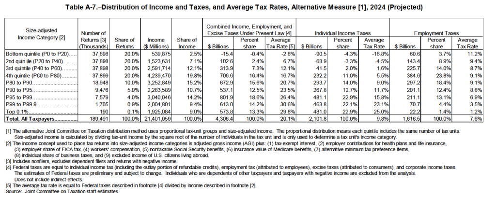
The following table from the JCT report is similar to the table in Chapter 17, which was based on data from the Tax Policy Center. The JCT report has the advantage of direct access to government tax data, which, as a private group, the Tax Policy Center doesn’t have. In addition, the JCT reports on an income group—the top 0.1 percent of income earners—compiled from government data not available to the Tax Policy Center. (Much political discussion has focused on the income earned and taxes paid by the top 1 percent of earners, which is a much larger group than the top 0.1 percent. We discuss the top 1 percent in the Apply the Concept, “Who Are the 1 Percent, and How Do They Earn Their Incomes,” in Microeconomics and Economics, Chaper 17, Section 17.4.)
The table shows data for the first four quntiles (or groups of 20 percent of taxpayers), with the highest quintile divided further. The table shows that the federal individual income tax is highly progressive, with the two lowest income quintiles having negative average tax rates because they receive more in tax credits than they pay in taxes. Employment taxes—primarily the payroll tax used to fund the Social Security and Medicare Systems—are regressive, with the lowest deciles paying a larger percentage of their income in these taxes than do the higher deciles. The regressivity of employment taxes is the result of both payroll taxes being levied on the first dollar of wages and salaries individuals earn and the part of the payroll tax used to fund the Social Security system dropping to zero for incomes above a certain level—$168,600 in 2024. Because income taxes are much larger in total than employment taxes or excise taxes—such as the federal taxes on gasoline, airline tickets, and alcoholic beverages—the total of these three types of federal taxes is progressive, as shown by the fact that the average tax rate rises with income. (Although note that the top 0.1 percent pay taxes at a slightly lower rate than do the other taxpayers included in the top 1 percent.)
USC quarterback Caleb Williams is shown with NFL Commissioner Roger Goodell at the NFL college draft in Detroit. (Photo from Reuters via the Wall Street Journal)
In late April, the National Football League (NFL) held its annual draft of eligible college players. NFL teams choose players through seven rounds in reverse order of how the teams finished in the previous year: The team with the worst record picks first and the winner of the Super Bowl picks last. Teams are allowed to trade picks with each other. This year, although the Carolina Panthers finished with the worst record during the 2023 season, they had traded their first round pick to the Chicago Bears, who picked first.
The Bears choose University of Southern California (USC) quarterback Caleb Williams with the first pick in the draft. Drafted players usually have no choice but to sign contracts with the team that chose them. A player can refuse to sign with the team that drafted him and not play that year, hoping that the next year a team they like better will draft them. Very few players have chosen that option.
When football fans and sportswriters discuss whether a team is a good match for a player they usually focus on factors such as whether a player’s skills are well suited to the team’s style of play and on how many other good players are on the team. One other factor that is seldom discussed is whether a player will benefit more financially by playing for the team that drafted him rather than for another team. Players chosen in the college draft are paid an amount fixed as a result of bargaining between the NFL and the National Football League Players Association (NFLPA), which is the labor union that represents NFL players.
As the first pick in the draft, Caleb Williams’s contract will pay him $39.4 million in total over the next four seasons. A sizeable fraction of that amount—probably $25.5 million—will be in the form of a lump-sum bonus that the Bears will pay Williams in full when he signs his contract. The dollar amount Williams is paid as the first pick in the draft would be the same whichever of the 32 NFL teams had drafted him. However, football players—like everyone else—are interested in their after-tax income and state and local income tax rates vary widely. Football players pay state and local income taxes based on where their teams’ games are played. In the 17-game NFL schedule, teams play either 8 or 9 games in their home city and the rest (road games) in the home cities of their opponents.
Jared Walczak of the Tax Foundation has compiled a table showing the tax rate each NFL team’s players will pay in 2024 based on the state and local taxes levied in their home city and the state and local taxes levied by the cities where the team’s road games will be played. To keep the numbers simple, let’s look at how the much in taxes Williams will owe on a $20 million bonus, which the Bears will pay him as soon as he signs his contract. (Note that, as indicated earlier, Williams’s bonus is likely to be greater than $20 million and he will also receive a salary during his first season of about $3.75 million.)
Given the income tax rate levied by the state of Illinois (the city of Chicago doesn’t levy a tax on income) and the state and local taxes levied by the cities and states in which the Bears will play their road games this year, Williams will owe a tax of $1,079,075 on his bonus. (Note that we are ignoring the substantial federal income tax that Williams will owe on the bonus because the federal tax won’t change no matter which city he plays in.) The lowest tax that Williams would pay on the bonus is $120,421, which would be his tax if he played for the Jacksonville Jaguars. Neither the city of Jacksonville nor the state of Florida levies a personal income tax, so Williams would only owe state and local income taxes on what he earns playing in cities where the Jaguars play their road games. The largest tax Williams would pay is $1,301,028, which would be his tax if he had been drafted by any of the three teams that play in California: the Los Angeles Rams, the Los Angeles Chargers, or the San Francisco ’49ers.
Although college players who are drafted are obliged to play for the team that drafted them, after players have completed their contracts they have the option of signing with a different team. At that stage of their careers, players—and their agents—can take into account state and local income taxes when deciding which team to sign a new contract with.
Supports: Microeconomics and Economics, Chapter 12, and Essentials of Economics, Chapter 9.
Photo from the Wall Street Journal.
A recent article in the Los Angeles Times discussed the problems faced by the owners of a sandwich shop in the Chinatown neighborhood of Los Angeles. The owners had closed the shop and then decided to reopen it. The article quoted one of the owners as saying: “After closing [the shop] we realized we still have our lease, we still have our loans from the [federal government’s Small Business Association], from COVID, the bills are still coming in. We can’t even afford to close. We can’t afford to be open, we can’t afford to be closed.”
a. What does the owner of the sandwich shop mean by saying they can’t afford to be open but they also can’t afford to be closed? Answer by explaining what the likely relationship is between the revenue the owners were earning from the shop and the shop’s fixed, variable, and total costs .
b. Are the owners likely to keep the sandwich shop open in the long run? Briefly explain.
Solving the Problem
Step 1: Review the chapter material. This problem is about when a firm should decide to shut down in the short run, so you may want to review the section “Deciding Whether to Produce or to Shut Down in the Shortrun” in Microeconomics (and Economics), Chapter 12, Section 12.4, (Essentials of Economics, Chapter 9, Section 9.4).
Step 2: Answer part a. by explaining what the sandwich shop’s owner meant by her statement, using the likely relationship between the shop’s revenue and its fixed, variable, and total cost in your explanation. That the owner states that “we can’t afford to be open” indicates that the firm is incurring a loss, so the revenue from the shop is less than the toal cost of operating it. But after closing the shop, the owners reopened it because “we can’t afford to be closed.” That statement indicates that the owners will incur a smaller loss by operating the shop than by keeping it closed. If the shop is closed, the owners still have to pay the shop’s fixed costs, such as the rent on the shop and the payments the owners must make on loans. We can infer that the loss from remaining open is less than the loss from being closed. In that situation, the shop’s revenue must be enough to cover the variable cost of operating it, although not enough to cover the total cost.
Step 3: Answer part b. by explaining whether the owners are likely to keep the sandwich shop open in the long run. By definition, in the long run, the owners will no longer have any fixed costs because the period of its lease will have ended and it will have paid off its loans—or possibly defaulted on them. If the revenue from operating the shop remains less than the total cost of operating it in the long run, the owners will permanenly close the shop.