Supports: Microeconomics and Economics, Chapter 6, and Essentials of Economics, Chapter 7.
Photo from from Reuters via the Wall Street Journal.
An article on bloomberg.com noted that in China after Apple cut by 10 percent the price of its iPhone 15 Pro Max—the most expensive iPhone model—sales of this model increased by 12 percent.
a. Based on this information, is the demand in China for this model iPhone price elastic or price inelastic? Briefly explain.
b. Do you have enough information to be confident in your answer to part a.? Briefly explain.
c. Assuming that the price elasticity you calculated in part a. is accurate, should managers at Apple be confident that if they cut the price of this iPhone model by an additional 10 percent they would sell 12 percent more? Briefly explain.
Solving the Problem
Step 1: Review the chapter material. This problem is about the price elasticity of demand, so you may want to review Microeconomics (and Economics), Chapter 6, Sections 6.1, 6.2 and 6.3 (Essentials of Economics, Chapter 7, Sections 7.5, 7.6, and 7.7)
Step 2: Answer part a. by using the information provided to determine whether the demand for this iPhone model in China is price elastic or price inelastic. In Section 6.1, we define the price elasticity of demand as being equal to (Percentage change in quantity demanded)/(Percentage change in price). From the information given, the price elasticity of demand for this iPhone model in China equals 12%/–10% = –1.2. Because this value is greater than 1 in absolute value, we can conclude that demand for this iPhone model in China is price elastic.
Step 3: Answer part b. by discussing whether you have enough information to be confident in your answer to part a. If we have values for the change in price and the change in the quantity demanded, we can calculate the price elasticity of demand provided that nothing that would affect the willingness of consumers to buy the good—other than the price of the good—has changed. In this case, if other factors that are relevant to consumers in making their decision about buying that iPhone model have changed, then the demand curve will have shifted and the 12 percent increase in iPhones sold will be a mixture of the effect of the price having decreased and the effects of other factors having changed. For example, if the prices of smartphones sold by Vivo and Huawei—two Chinese firms whose smartphones compete with the iPhone—had increased, then the demand curve for the iPhone 15 Pro Max will have shifted to the right and our calculation in part a. will not give us an accurate value for the price elasticity of demand for the iPhone 15 Pro Max.
Step 4: Answer part c. by explaining whether, assuming that the price elasiticity you calculated in part a. is accurate, Apple’s managers can be confident that if they if they cut the price of this iPhone model by an additional 10 percent they would sell 12 percent more of this model. The first price cut for this iPhone model caused a movement down the demand curve. For Apple’s managers to be confident that that the same percentage price cut would result in the same percentage increase in the quantity sold, the price elasticity would have to be constant along the demand curve for this model. As we show explicitly for a linear demand curve in Section 6.3, the price elasticity of demand is unlikely to be constant along the demand curve (although in an unusual case it would be). In general, we expect that in moving further down the demand curve the price elasticity of demand will decline in absolute value. If that result holds in this case, then an additional 10 percent cut in price is likely to result in less than a 12 percent increase in the quantity demanded.
Chair Jerome Powell at a meeting of the Federal Open Market Committee (photo from federalreserve.gov)
At the beginning of the year, there was an expectation among some economists and policymakers that the Fed’s policy-making Federal Open Market Committee (FOMC) would begin cutting its target range for the federal funds rate at the meeting that ended today (May 1). The Fed appeared to be bringing the U.S. economy in for a soft landing—inflation returning to the Fed’s 2 percent target without a recession occurring.
During the first quarter of 2024, production and employment have been expanding more rapidly than had been expected and inflation has been higher than expected. As a result, the nearly universal expectation prior to this meeting was that the FOMC would leave its target for the federal funds rate unchanged. Some economists and investment analysts have begun discussing the possiblity that the committee might not cut its target at all during 2024. The view that interest rates will be higher for longer than had been expected at the beginning of the year has contributed to increases in long-term interest rates, including the interest rates on the 10-year Treasury Note and on residential mortgage loans.
The statement that the FOMC issued after the meeting confirmed the consensus view:
“Recent indicators suggest that economic activity has continued to expand at a solid pace. Job gains have remained strong, and the unemployment rate has remained low. Inflation has eased over the past year but remains elevated. In recent months, there has been a lack of further progress toward the Committee’s 2 percent inflation objective.”
In his press conference after the meeting, Fed Chair Jerome Powell emphasized that the FOMC was unlikely to cut its target for the federal funds rate until data indicated that the inflation rate had resumed falling towards the Fed’s 2 percent target. At one point in the press conference Powell noted that although it was taking longer than expected for the inflation rate to decline he still expected that the pace of economic actitivity was likely to slow sufficiently to allow the decline to take place. He indicated that—contrary to what some economists and investment analysts had suggested—it was unlikely that the FOMC would raise its target for the federal funds rate at a future meeting. He noted that the possibility of raising the target was not discussed at this meeting.
Was there any news in the FOMC statement or in Powell’s remarks at the press conference? One way to judge whether the outcome of an FOMC meeting is consistent with the expectations of investors in financial markets prior to the meeting is to look at movements in stock prices during the time between the release of the FOMC statement at 2 pm and the conclusion of Powell’s press conference at about 3:15 pm. The following figure from the Wall Street Journal, shows movements in the three most widely followed stock indexes—the Dow Jones Industrial Average, the S&P 500, and the Nasdaq composite. (We discuss movements in stock market indexes in Macroeconomics and Essentials of Economics, Chapter 6, Section 6.2 and in Economics, Chapter 8, Section 8.2.)
If either the FOMC statement or the Powell’s remarks during his press conference had raised the possibility that the committee was considering raising its target for the federal funds rate, stock prices would likely have declined. The decline would reflect investors’ concern that higher interest rates would slow the economy, reducing future corporate profits. If, on the other hand, the statement and Powell’s remarks indicated that the committee would likely cut its target for the federal funds rate relatively soon, stock prices would likely have risen. The figure shows that stock prices began to rise after the 2 pm release of the FOMC statement. Prices rose further as Powell seemed to rule out an increase in the target at a future meeting and expressed confidence that inflation would resume declining toward the 2 percent target. But, as often happens in the market, this sentiment reversed towards the end of Powell’s press conference and two of the three stock indexes ended up lower at the close of trading at 4 pm. Presumably, investors decided that on reflection there was no news in the statement or press conference that would change the consensus on when the FOMC might begin lowering its target for the federal funds rate.
The next signficant release of macroeconomic data will come on Friday when the Bureau of Labor Statistics issues its employment report for April.
One of the key lessons of economics is that competition serves to push firms toward serving the interests of consumers. When existing firms in an industry are making an economic profit, new firms will enter the industry, which increases the quantity of the good produced and lowers the good’s price. Entry is the essential mechanism that drives a competitive market economy towards achieving allocative efficiency—with the mix of goods and services produced matching consumer preferences—and productive efficiency—with goods and services being produced at the lowest possible cost. (We discuss allocative efficiency and productive efficiency in Chapter 1, Section 1.2.)
For entry to occur requires the efforts of entrepreneurs, who constantly search for opportunities to make a profit. (We discuss the role of entrepreneurs in a market economy in Chapter 2, Section 2.3.) Although, not well remembered today, Victor S. Fox was one of the more flamboyant entrepreneurs in U.S. business history. Fox was born in England in 1893 and moved with his family to Massachusetts three years later. As a young man, he started a firm to manufacture women’s clothing. In 1917, with the entry of the United States into World War I, Fox’s firm switched to producing military uniforms. In 1920, after the end of the war, Fox founded Consolidated Maritime Lines to buy from the U.S. government confiscated German and Austrian cargo ships. Fox also purchased a coal mine in Virginia to provide fuel for the ships. This effort ended in bankruptcy.
In 1929, Fox founded Allied Capital Corporation to invest in the stock market. This firm also failed amid accusations that Fox had broken securities laws. (Most of the information on Fox’s early career is from this site, which relies primarily on mentions of Fox in newspapers.) In 1936, Fox founded Fox Feature Syndicate to produce magazines. At that point, very few comic books were being published. That changed in April 1938, when National Allied Publications released Action Comics, featuring Superman—generally considered the first superhero to appear in comic books. Sales of Superman comic books soared and Fox responded by entering the comic book industry, publishing a comic book starring Wonder Man. Wonder Man was an obvious copy of Superman, which led Superman’s publisher to file a lawsuit against Fox for copyright infringement. Fox agreed to stop publishing Wonder Man, but continued to publish comic books starring superheroes who weren’t such obvious copies of Superman.
As this summary of Fox’s career indicates, he was an entrepreneur who was willing to enter a new industry whenever he saw a profit opportunity, even if he lacked previous experience in the industry. In 1941, the continuing success of Coca-Cola and Pepsi-Cola led Fox to attempt to enter the cola industry in what was his most audacious entrepreneurial effort. The high sales of his comic books gave Fox a platform to advertise his new soft drink —Kooba cola. The following are some of Fox’s advertisements for Kooba cola.
Fox also advertised Kooba on a radio program featurning the Blue Beetle, one of his comic book superheroes. In the print advertisements for Kooba, Fox seems to have focused on two points in an attempt to differentiate his cola from existing colas, particularly Coke and Pepsi. (We discuss the role product differentiation plays in competition among firms in Microeconomics and Economics, Chapter 13.) First, to help overcome the belief among some consumers that colas were an unhealthy drink, Fox emphasized that Kooba cola would contain vitamin B1. In 1941, vitamin B1 had only recently become available and was the subject of newspaper stories. Second, at 12 ounces, bottles of Kooba were nearly twice as large as the standard 6.5 ounce Coke bottle but would sell for the same 5 cent price. One of the advertisements above notes that a six-pack of Kooba had a price of only 25 cents.
How was Fox able to sell his new cola for about half the price per ounce of Coke or Pepsi? That’s unclear because—amazingly—at the time Fox was running these advertisements, not only was Kooba not “available everywhere,” as the advertisements claimed, it wasn’t available anywhere. Fox was heavily advertising a product that didn’t actually exist.
How did Fox hope to earn a profit selling a nonexistent product? Fox’s strategy was apparently to begin by heavily advertising Kooba in the hopes of sparking a demand for it. He seems to have believed that if enough people were inspired by his advertisements to ask for the cola at grocery stores and newsstands, he could approach an existing soft drink company and offer to license the Kooba name. He seems never to have intended to actually manufacture the cola, relying instead on royalties paid by the soft drink company he hoped to license the name to.
Perhaps unsurprisingly, Fox’s strategy failed. To capitalize on Fox’s advertising, a firm licensing the Kooba name would have had to find a way to make a profit despite selling the cola at a price about half the price charged by competitors. Because Fox had no experience in manufacturing colas, he presumably had no advice to give on how production costs could be reduced sufficiently to allow Kooba to be sold at a profit.
Fox engaged in other entrepreneurial efforts before passing away in 1957. Over the years, Fox pursued a number of business strategies, some of which were successful, at least for a time. But his attempt to make a profit by promoting a nonexistent cola ranks among the the most dubious strategies in U.S. business history. A strategy that likely left some consumers puzzled that a cola that appeared in advertisements was never available in store.
This op-ed orginally appeared in the Wall Street Journal.
Put Growth Back on the Political Agenda
In a campaign season dominated by the past, a central economic topic is missing: growth. Rapid productivity growth raises living standards and incomes. Resources from those higher incomes can boost support for public goods such as national defense and education, or can reconfigure supply chains or shore up social insurance programs. A society without growth requires someone to be worse off for you to be better off. Growth breaks that zero-sum link, making it a political big deal.
So why is the emphasis on growth fading? More than economics is at play. While progress from technological advances and trade generally is popular, the disruption that inevitably accompanies growth and hits individuals, firms and communities has many politicians wary. Such concerns can lead to excessive meddling via industrial policy.
As we approach the next election, the stakes for growth are high. Regaining the faster productivity that prevailed before the global financial crisis requires action. The nonpartisan Congressional Budget Office estimates potential gross domestic product growth of 1.8% over the coming decade, and somewhat lower after that. Those figures are roughly 1 percentage point lower than the growth rate over the three decades before the pandemic. Many economists believe productivity gains from generative artificial intelligence can raise growth in coming decades. But achieving those gains requires an openness to change that is rare in a political climate stuck in past grievances about disruption—the perennial partner of growth.
Traditionally, economic policy toward growth emphasized support for innovation through basic research. Growth also was fostered by reducing tax burdens on investment, streamlining regulation (which has proliferated during the Biden administration) and expanding markets. These important actions have flagged in recent years. But such attention, while valuable, masks inattention to adverse effects on some individuals and communities, raising concerns about whether open markets advance broad prosperity.
This opened a lane for backward-looking protectionism and industrial policy from Democrats and Republicans alike. Absent strong national-defense arguments (which wouldn’t include tariffs on Canadian steel or objections to Japanese ownership of a U.S. steel company), protectionism limits growth. According to polls by the Chicago Council on Global Affairs, roughly three-fourths of Americans say international trade is good for the economy. Finally, protectionism belies ways in which gains from openness may be preserved, such as by simultaneously offering support for training and work for communities of individuals buffeted by trade and technological change.
On industrial policy, it is true that markets can’t solve every allocation problem. But such concerns underpin arguments for greater federal support of research for new technologies in defense, climate-change mitigation, and private activity, not micromanaged subsidies to firms and industries. If a specific defense activity merits assistance, it could be subsidized. These alternatives mitigate the problems in conventional industrial policy of “winner picking” and, just as important, the failure to abandon losers. It is policymakers’ hyperattention to those buffeted by change that hampers policy effectiveness and, worse, invites rent-seeking behavior and costly regulatory micromanagement.
Examples abound. Appending child-care requirements to the Chips Act and the inaptly named Inflation Reduction Act has little to do with those laws’ industrial policy purpose. The Biden administration’s opposition to Nippon Steel’s acquisition of U.S. Steel raises questions amid the current wave of industrial policy. How is a strong American ally’s efficient operation of an American steel company with U.S. workers an industrial-policy problem? Flip-flops on banning TikTok fuel uncertainty about business operations in the name of industrial policy.
The wrongly focused hyperattention is supposedly grounded in putting American workers first. But it raises three problems. First, the interventions raise the cost of investments, and the jobs they are to create or protect, by using mandates and generating policy uncertainty. Second, they contradict the economic freedom in market economies of voluntary transactions. Absent a strong national-security foundation, why is public policy directing investment in or ownership of assets? Such policies threaten the nation’s long-term prosperity by discouraging investment and invite rent-seeking in a way that voluntary market transactions don’t. Both problems hamstring growth.
Third, and perhaps most important, such micromanagement misses the economic and political mark of actually helping individuals and communities disrupted by growth-enhancing openness. A more serious agenda would focus on training suited to current markets (through, for example, more assistance to community colleges), on work (through expanding the Earned Income Tax Credit), and on aid to communities hit by prolonged employment loss (through services that enhance business formation and job creation). The federal government could also establish research centers around the country to disseminate ideas for businesses.
Growth matters—for individual livelihoods, business opportunities and public finances. Pro-growth policies that account for disruption’s effects while encouraging innovation, saving, capital formation, skill development and limited regulation must return to the economic agenda. A shift to prospective, visionary thinking would reorient the bipartisan, backward-looking protectionism and industrial policy that weaken growth and fail to address disruption.
Supports:Macroeconomics, Chapter 5, Section 5.3 or Chapter 6, Section 6.1; Microeconomics and Economics, Chapter 7, Section 7.3 or Chapter 8, Section 8.1.
Image from Reuters via the Wall Street Journal.
A recent paper by Iyah Rahwan, of the Max Planck Institute for Human Development in Berlin Germany, and colleagues raises the possibility that dating apps, like Tinder, OkCupid, and Bumble, may have a principal-agent problem. Dating apps—like nearly all other subscription apps—generate more income if subscribers pay for the app over a longer period of time. Many people use dating apps in the hope of connecting with another app user with whom they can have a long-term relationship.
a. What is the principal-agent problem?
b. Explain whether dating apps may have a principal-agent problem. If they do, who is the principal and who is the agent?
c. How does your answer to part b. affect your estimate of how likely people using dating apps are to find a long-term relationship using these apps?
Solving the Problem
Step 1:Review the chapter material. This problem is about the principal-agent problem, so you may want to review either of the two sections in which the principal-agent problem is discussed: Macroeconomics, Chapter 5, Section 5.3, “Information Problems and Externalities in the Market for Health Care” or Chapter 6, Section 6.1, “Types of Firms” (Microeconomics and Economics, Chapter 7, Section 7.3 or Chapter 8, Section 8.1.)
Step 2:Answer part a. by defining “principal-agent” problem. Principal-agent is defined in the textbook this way: A problem caused by an agent pursuing the agent’s own interests rather than the interests of the principal who hired the agent.
Step 3: Answer part b. by explaining why dating apps may have a principal-agent problem and by identifying who is the principal and who is the agent in this situation. With dating apps, the principal is the app user who, typically, uses the app to help find a partner for a long-term relationship. The owners of the dating app are the agent because they have been hired by the app user to help the user achieve the goal of starting a long-term relationship. Unfortunately, the owners of the dating app have a different goal than does the app user. The goal of the owners is to have users keep subscribing to the app. Anyone who finds a long-term relationship using the app is likely (we hope!) to drop his or her subscription to the app. Therefore, whereas the app user would like to quickly find a partner for a long-term relationship, the owners of the app want the app user to take a long time to find such a partner.
Step 4: Answer part c. by discussing how the principal-agent problem may affect the likelihood of someone using a dating app successfully finding someone for a long-term relationship. The answer to part b. indicates that dating apps may have an incentive to make it somewhat more difficult to find a long-term relationship using the app—perhaps by employing a matching algorithm that doesn’t result in users easily finding good matches. Therefore, it’s likely that the principal-agent problem make it less likely that people using dating apps will successfully find a partner for a long-term relationship.
Source: Iyah Rahwan, et al., “Price of Anarchy in Algorithmic Matching of Romantic Partners,” ACM Transactions on Economics and Computation, Vol. 12, No. 1, pp. 1-25.
Supports: Microeconomics, Chapter 15, Section 15.6; Economics, Chapter 55, Section 15.6; and Essentials of Economics, Chapter 10, Sections 10.6.
PG&E workers moving a powerline underground. (Photo from the Wall Street Journal.)
PG&E, Southern California Edison, and San Diego Gas and Electric are public utilities that provide electricity and natural gas to households and firms in California. (For the most part, they provide these services in different parts of the state.) The California Public Utilities Commission regulates the prices that these utilities charge. In March 2024, an article in the San Francisco Chronicle reported that the commission proposed that the utilities begin charging households who receive their electricity from these utilities an additional flat fee of $24 per month (that would not depend on the quantity of electricity a household uses), while reducing the price households pay for each kilowatt hour they use by about 6 cents.
Isn’t this policy contradictory—adding a flat fee to households’ electric bills while reducing the price per kilowatt hour households pay? Can you explain why the policy might make economic sense? Draw a graph showing the situation of a public utility to illustrate your answer.
Solving the Problem
Step 1: Review the chapter material. This problem is about how the government regulates public utilities, so you may want to review the section in Microeconomics, Chapter 15, Section 15.6, on “Regulating Natural Monopolies,” (Economics, Chapter 15, Section 15.6 and Essentials of Economics, Chapter 10, Section 10.6).
Step 2: Explain why the policy isn’t contradictory and why it might make economic sense. It may seem as if the commission is being contradictory in imposing a new flat rate fee on households while at the same time lowering the price they pay per kilowatt hour used. But, as we discuss in Chapter 15, public utilities are typically natural monoplies because economies of scale are so large in that industy that one firm can supply the electricity in a market at a lower average cost than can two or more firms. Figure 15.1, reproduced below, shows this situation.
As we discuss in the “Regulating Monopoly” section of Chapter 15, Section 15.6, as a result of the large economies of scale in generating electricity, at the quantity at which the marginal cost curve crosses the demand curve, the marginal cost curve is below the demand curve. The economically efficient price is the price equal to the marginal cost of generating electricity. But if the public utility commission requires the utility to charge this price, the utility will suffer losses because it will not be covering its average total cost. The combination of charging households a flat fee while lowering the price they pay per kilowatt hour can help overcome this problem.
Step 3: Finishing solving the problem by drawing a graph to illustrate your answer. You should draw graph similar to Figure 18.8, which we reproduce below. In this graph, if the utility is required to charge the economically efficient price, PE, it will suffer a loss equal to red rectangle. As a result, public utility commissions often set the price of electricity equal to PR, but at that price households demand the quantity of electricity, QR, which is less than the economically efficient quantity, QE. Note, though, that if a public utility commission allows a utillity to collect a flat fee from households equal to the amount shown by the red rectangle, it can require the utility to charge the economically efficient price, PE.
The key point here is that, because it doesn’t change as the quantity of electricity generated and used changes, the flat fee doesn’t affect either the utility’s marginal cost of generating electricity or the cost to households of using another kilowatt of electricity.
We don’t know from the discussion in the article whether the flat fee will cover the entire amount of the utilities’ losses or if the new price will be equal to the efficient price. But the policy can still make economic sense if the new price is closer to the efficient price than was the previous price.
Source: Julie Johnson, “California Proposes A $24 Flat Fee on Utility Bills in Exchange for Lower Electricity Prices,” San Francisco Chronicle, March 28, 2024.
Wendy’s management intends to begin using dynamic pricings in its fast-food restaurants. As we discuss in Microeconomics and Economics, Chapter 15, Section 15.5 (Essentials of Economics, Chapter 10, Section 10.5), dynamic pricing is a form of price discrimination, which is the business practice of charging different prices to different customers for the same good or service. The ability of firms to analyze customer data using machine learning models has increased the ability to price discriminate.
One form of price discrimination involves charging customers different prices at different times, as, for instance, when movie theaters charge a lower price during afternoon showings than during evening showings. As a group, people who can choose whether to attend either an afternoon or an evening showing are more sensitive to changes in the price of a ticket—that is, their demand for tickets is more price elastic—than are people who can only attend an evening showing. Price discrimination with respect to movie tickets results in movie theaters earning a greater profit than if they charged the same price for all showings.
In a conference call with investors in February, Wendy’s CEO Kirk Tanner indicated that next year the firm would begin using dynamic pricing of its hamburgers and other menu items by charging different prices at different times of the day. Tanner didn’t provide details on how prices would differ in high demand times, such as during lunch and dinner, and low demand times, such as the middle of the afternoon. Some business commentators, though, assumed that Wendy’s dynamic pricing strategy would resemble Uber’s surge pricing strategy. As we discuss in Microeconomics, Economics, and Essentials of Economics, Chapter 4, Section 4.1, Uber increases prices during periods of high demand, such as on New Year’s Eve.
The idea that Wendy’s would increase prices at peak times sparked a strong reaction on social media with many people criticizing the firm for “price gouging.” Rival fast-food restaurants joined the criticism. Burger King posted on X (formerly Twitter) that “we don’t believe in charging people more when they’re hungry.” As we note in Microeconomics and Economics, Chapter 10, Section 10.3 (Essentials of Econmics, Chapter 7, Section 7.3), surveys indicate that many people believe that it is fair for firms to raise prices following an increase in the firms’ costs, but unfair to raise prices following an increase in demand.
One way for firms to avoid this reaction from consumers while still price discriminating is to frame the issue by stating that they charge regular prices during times of peak demand and discount prices during times of low demand. For example, recently one AMC theater was charging $13.99 for a 7:15 PM showing of Dune: Part Two, but a “Matinee Discount Price” of $10.39 for a 1:oo PM showing of the film. Note that there is no real economic difference between AMC calling the evening price the normal price and the afternoon price the discoung price and the firm calling the afternoon price the normal price and the evening price a “surge price.” But one of the lessons of behavioral economics is that firms should pay attention to how consumers intepret a policy. Many consumers clearly see the two pricing strategies as different even though economically they aren’t. (We discuss behavioral economics in Microeconomics and Economics, Chapter 10, Section 10.4, and in Essentials of Economics, Chapter 7, Section 7.4.)
Not surprisingly, following the adverse reaction to its annoucement that it would begin using dynamic pricing, Wendy’s responded with a blog post in which it stated that its new pricing strategy was “misconstrued in some media reports as an intent to raise prices when demand is highest at our restaurants. We have no plans to do that and would not raise prices when our customers are visiting us most.” And that: “Digital menuboards could allow us to change the menu offerings at different times of day and offer discounts and value offers to our customers more easily, particularly in the slower times of day.” In effect, Wendy’s was framing its pricing strategy the way movie theaters do rather than the way Uber does.
Wendy’s CEO probably realizes now that how a pricing strategy is presented to consumers can affect how successful the strategy will be.
Supports: Microeconomics and Economics, Chapter 12, and Essentials of Economics, Chapter 9.
The entrance to the Lincoln Tunnel, which connects New Jersey to Midtown Manhattan. (Photo from the Associated Press via the New York Times.)
This spring, New York City will begin charging an additional fee—referred to as a congestion price or congestion toll—on vehicles entering the borough of Manhattan below 60th Street. The purpose of the fee is to reduce the congestion and pollution that additional vehicles cause when driving in that part of the city. (Note that the fee can be thought of as Pigovian tax because it is intended to address a negative externality caused by driving a vehicle. We discuss Pigovian taxes in Microeconomics and Economics, Chapter 5, Section 5.3, and in Essentials of Economics, Chapter 4, Section 4.5.)
Trans-Bridge Lines operates buses between the Lehigh Valley in Pennsylvania and Manhattan. The firm will have to pay a fee of $24 each time one of its buses enters Manhattan. An article in the (Allentown, PA) Morning Call quotes the president of Trans-Bridge Lines as objecting to the fee: “It doesn’t make sense and punishes bus operators who are part of the solution to the congestion problem.” However, the article also notes that “Trans-Bridge is not considering fare increases at this time.”
If Trans-Bridge’s cost of providing bus service between the Lehigh Valley and Manhattan increases by $24 per bus, shouldn’t the firm raise the price it charges passengers? Does the failure of Trans-Bride to raise ticket prices following the enactment of the fee mean that the firm isn’t its maximizing profit? Briefly explain.
Solving the Problem
Step 1:Review the chapter material.This problem is about what costs firms take into account when determining the profit-maximizing price to charge in the short run, so you may want to review Microeconomics or Economics, Chapter 12, Section 12.2, “How a Firm Maximizes Profit in a Perfectly Competitive Market” (Essentials of Economics, Chapter 9, Section 9.2)
Step 2:Answer the two questions by explaining what type of cost the $24 fee is and whether the fee should affect the profit-maximizine price Trans-Bridge Lines should charge passengers for a ticket on a bus going to Manhattan. The fee is a flat $24 per bus and, so, it doesn’t change with the number of passengers on a bus. Therefore, the fee is a fixed cost to Trans-Bridge. Trans-Bridge should set the price of a ticket so that the last ticket sold on a bus increases the firm’s marginal cost and marginal revenue by the same amount. Because the $24 fee doesn’t change the marginal cost (or the marginal revenue) to the firm of transporting another passenger, the fee doesn’t change the firm’s profit-maximizing price. The answer to the first question in the problem is that an increase (or decrease) in a firm’s fixed cost won’t cause the firm to change its profit-maximizing price in the short run. The answer to the second question follows from the answer to the first question: That Trans-Bridge isn’t raising the price of a ticket following the enactment of the doesn’t mean that the firm isn’t maximizing profit.
Extra credit: Note that in the answer we refer to Trans-Bridge’s decision in the short run. It’s possible that the $24 fee will cause Trans-Bridge to suffer an economic loss on at least some of the bus trips it offers during different times during the day. As we discuss in Microeconomics and Economics, Chapter 12, Section 12.4 (Essentials of Economics, Chapter 9, Section 9.4), in that case, Trans-Bridge will continue to offer those bus trips in the short run, but, if nothing else changes, it will stop offering the trips in the long run.
Recent articles in the business press have discussed the possibility that the U.S. economy is entering a period of higher growth in labor productivity:
“US Productivity Is on the Upswing Again. Will AI Supercharge It?” (link)
“Can America Turn a Productivity Boomlet Into a Boom?” (link)
In Macroeconomics, Chapter 16, Section 16.7 (Economics, Chapter 26, Section 26.7), we highlighted the role of growth in labor productivity in explaining the growth rate of real GDP using the following equations. First, an identity:
Real GDP = Number of hours worked x (Real GDP/Number of hours worked),
where (Real GDP/Number of hours worked) is labor productivity.
And because an equation in which variables are multiplied together is equal to an equation in which the growth rates of these variables are added together, we have:
Growth rate of real GDP = Growth rate of hours worked + Growth rate of labor productivity
From 1950 to 2023, real GDP grew at annual average rate of 3.1 percent. In recent years, real GDP has been growing more slowly. For example, it grew at a rate of only 2.0 percent from 2000 to 2023. In February 2024, the Congressional Budget Office (CBO) forecasts that real GDP would grow at 2.0 percent from 2024 to 2034. Although the difference between a growth rate of 3.1 percent and a growth rate of 2.0 percent may seem small, if real GDP were to return to growing at 3.1 percent per year, it would be $3.3 trillion larger in 2034 than if it grows at 2.0 percent per year. The additional $3.3 trillion in real GDP would result in higher incomes for U.S. residents and would make it easier for the federal government to reduce the size of the federal budget deficit and to better fund programs such as Social Security and Medicare. (We discuss the issues concerning the federal government’s budget deficit in this earlier blog post.)
Why has growth in real GDP slowed from a 3.1 percent rate to a 2.0 percent rate? The two expressions on the right-hand side of the equation for growth in real GDP—the growth in hours worked and the growth in labor productivity—have both slowed. Slowing population growth and a decline in the average number of hours worked per worker have resulted in the growth rate of hours worked to slow substantially from a rate of 2.0 percent per year from 1950 to 2023 to a forecast rate of only 0.4 percent per year from 2024 to 2034.
Falling birthrates explains most of the decline in population growth. Although lower birthrates have been partially offset by higher levels of immigration in recent years, it seems unlikely that birthrates will increase much even in the long run and levels of immigration also seem unlikely to increase substantially in the future. Therefore, for the growth rate of real GDP to increase significantly requires increases in the rate of growth of labor productivity.
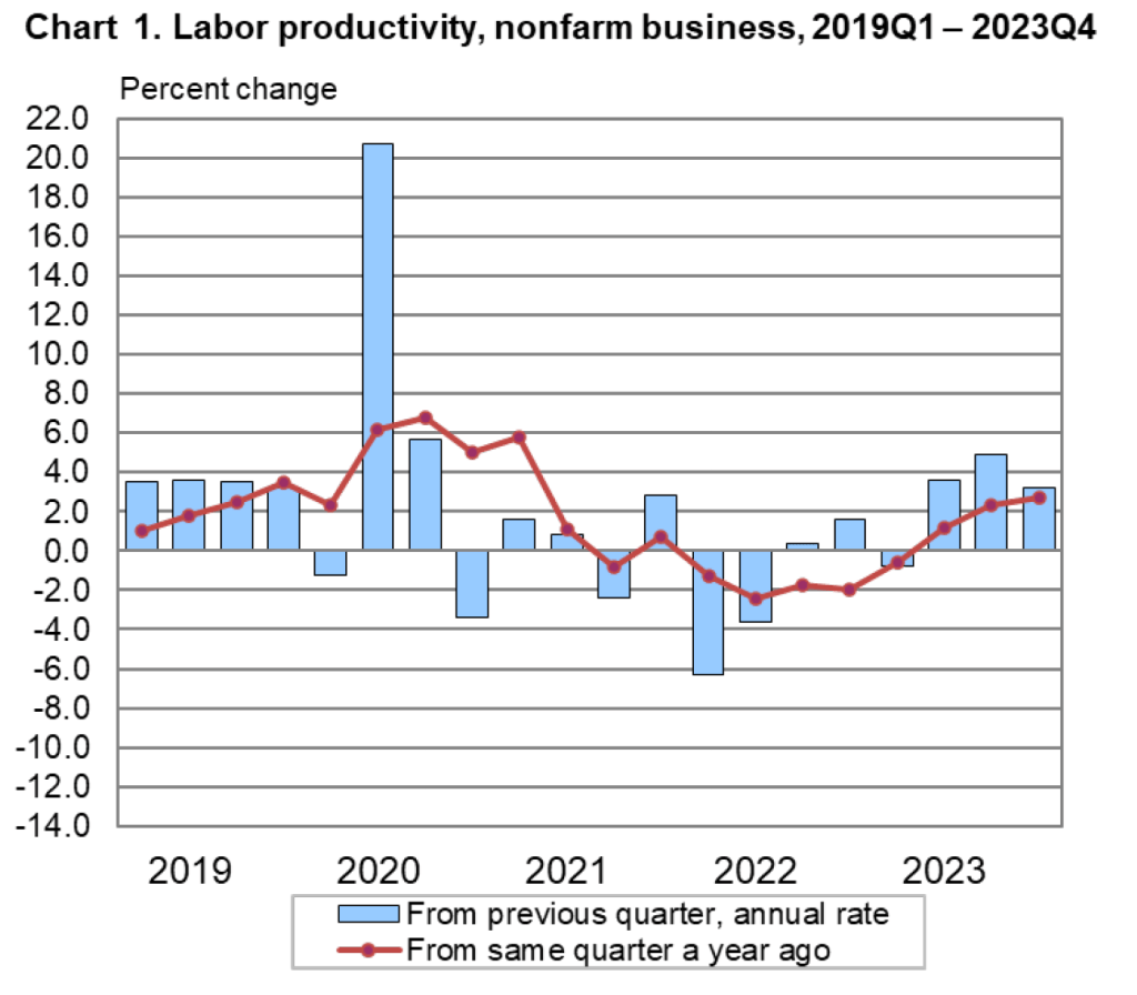
The Bureau of Labor Statistics (BLS) publishes quarterly data on labor productivity. (Note that the BLS series is for labor productivity in the nonfarm business sector rather than for the whole economy. Output of the nonfarm business sector excludes output by government, nonprofit businesses, and households. Over long periods, growth in real GDP per hour worked and growth in real output of the nonfarm business sector per hour worked have similar trends.) The following figure is taken from the BLS report “Productivty and Costs,” which was released on February 1, 2024.
Note that the growth in labor productivity increased during the last three quarters of 2023, whether we measure the growth rate as the percentage change from the same quarter in the previous year or as growth in a particular quarter expressed as anual rate. It’s this increase in labor productivity during 2023 that has led to speculation that labor productivity might be entering a period of higher growth. The following figure shows labor productivity growth, measured as the percentage change from the same quarter in the previous year for the whole period from 1950 to 2023.
The figure indicates that labor productivity has fluctuated substantially over this period. We can note, in particular, productivity growth during two periods: First, from 2011 to 2018, labor productivity grew at the very slow rate of 0.9 percent per year. Some of this slowdown reflected the slow recovery of the U.S. economy from the Great Recession of 2007-2009, but the slowdown persisted long enough to cause concern that the U.S. economy might be entering a period of stagnation or very slow growth.
Second, from 2019 through 2023, labor productivity went through very large swings. Labor productivity experienced strong growth during 2019, then, as the Covid-19 pandemic began affecting the U.S. economy, labor productivity soared through the first half of 2021 before declining for five consecutive quarters from the first quarter of 2022 through the first quarter of 2023—the first time productivity had fallen for that long a period since the BLS first began collecting the data. Although these swings were particularly large, the figure shows that during and in the immediate aftermath of recessions labor productivity typically fluctuates dramatically. The reason for the fluctuations is that firms can be slow to lay workers off at the beginning of a recession—which causes labor productivity to fall—and slow to hire workers back during the beginning of an economy recovery—which causes labor productivity to rise.
Does the recent increase in labor productivity growth represent a trend? Labor productivity, measured as the percentage change since the same quarter in the previous year, was 2.7 percent during the fourth quarter of 2023—higher than in any quarter since the first quarter of 2021. Measured as the percentage change from the previous quarter at an annual rate, labor productivity grew at a very high average rate of 3.9 during the last three quarters of 2023. It’s this high rate that some observers are pointing to when they wonder whether growth in labor productivity is on an upward trend.
As with any other economic data, you should use caution in interpreting changes in labor productivity over a short period. The productivity data may be subject to large revisions as the two underlying series—real output and hours worked—are revised in coming months. In addition, it’s not clear why the growth rate of labor productivity would be increasing in the long run. The most common reasons advanced are: 1) the productivity gains from the increase in the number of people working from home since the pandemic, 2) businesses’ increased use of artificial intelligence (AI), and 3) potential efficiencies that businesses discovered as they were forced to operate with a shortage of workers during and after the pandemic.
To this point it’s difficult to evaluate the long-run effects of any of these factors. Wconomists and business managers haven’t yet reached a consensus on whether working from home increases or decreases productivity. (The debate is summarized in this National Bureau of Economic Research Working Paper, written by Jose Maria Barrero of Instituto Tecnologico Autonomo de Mexico, and Steven Davis and Nicholas Bloom of Stanford. You may need to access the paper through your university library.)
Many economists believe that AI is a general purpose technology (GPT), which means that it may have broad effects throughout the economy. But to this point, AI hasn’t been adopted widely enough to be a plausible cause of an increase in labor productivity. In addition, as Erik Brynjolfsson and Daniel Rock of MIT and Chad Syverson of the University of Chicago argue in this paper, the introduction of a GPT may initially cause productivity to fall as firms attempt to use an unfamiliar technology. The third reason—efficiency gains resulting from the pandemic—is to this point mainly anecdotal. There are many cases of businesses that discovered efficiencies during and immediately after Covid as they struggled to operate with a smaller workforce, but we don’t yet know whether these cases are sufficiently common to have had a noticeable effect on labor productivity.
So, we’re left with the conclusion that if the high labor productivity growth rates of 2023 can be maintained, the growth rate of real GDP will correspondingly increase more than most economists are expecting. But it’s too early to know whether recent high rates of labor productivty growth are sustainable.
Action Comics No. 1, published in June 1938, is often consider the first superhero comic book. (Image from comics.org.)
In a political advertisement that ran before the broadcast of the Super Bowl, President Joe Biden discussed shrinkflation, which refers to firms reducing the quantity of a product in container while keeping the price unchanged. In this post from the summer of 2022, we discussed examples of shrinkflation—including Chobani reducing the quantity of yogurt in the package shown here from 5.3 ounces to 4.5 ounces—and noted that shrinkflation complicates the job of the Bureau of Labor Statistics when compiling the consumer price index.
This yogurt remained the same price although the quantity of yogurt in the container shrank from 5.3 ounces to 4.5 ounces.
Shrinkflation isn’t new; firms have used the strategy for decades. Firms are particularly likely to use shrinkflation during periods of high inflation or during periods when the federal government implements price controls. Firms also sometimes resort to shrinkflation when the the price of a product has remained constant for long enough that the firms fear that consumers will react strongly to the firms increasing the price.
Comic books provide an interesting historical example of shrinkflation. David Palmer, a professor of management at South Dakota State University published an article in 2010 in which he presented data on the price and number of pages in copies of Action Comics from 1938 to 2010. When DC Comics introduced Superman in the first issue of Action Comics in June 1938, it started the superhero genre of comic books. Action Comics No. 1 had a price of $0.10 and was 64 pages.
After the United States entered World War II in December 1941, the federal government imposed price controls to try to limit the inflation caused by the surge in spending to fight the war. Rising costs of producing comic books, combined with the difficulty in raising prices because of the controls, led comic book publishers to engage in shrinkflation. In 1943, the publishers reduced the number of pages in their comics from 64 to 56. In 1944, the publishers engaged in further shrinkflation, reducing the number of pages from 56 to 48.
In 1951, during the Korean War, the federal government again imposed price controls. Comic book publishers responded with further shrinkflation, keeping the price at $0.10, while reducing the number of pages from 48 to 40. In 1954, they shrank the number of pages to 36, which remains the most common number of pages in a comic book today. At that time, the publishers also slightly reduced the width of comics from 7 3/4 inches to 7 1/8 inches. (Today the typical comic book has a width of 6 7/8 inches.)
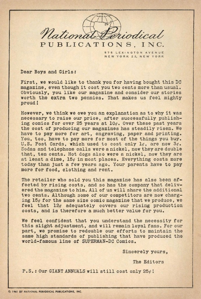
By the late 1950s, comic book publishers became convinced that they would be better off raising the prices of comic books rather than further shrinking the number of pages. But they were reluctant to raise their prices because they had been a constant $0.10 for more than 20 years, so children and their parents might react very negatively to a price increase, and because no firm wanted to be the first to raise its price for fear of losing sales to its competitors. They were caught in a prisoner’s dilemma: Comic book publishers would all have been better off if they had raised their prices but the antitrust laws kept them from colluding to raise prices and no individual firm had an incentive to raise prices alone. (We discuss collusion, prisoner’s dilemmas, and other aspects of oligopolistic firm behaviour in Chapter 14 of Microeconomics and Economics.)
The most successful publisher in the 1950s was Dell, which sold very popular comic books featuring Donald Duck, Uncle Scrooge, and other characters that particularly appealed to younger children. Because the prices of Dell’s comic books, like those of other publishers, been unchanged at $0.10 since the late 1930s, the firm didn’t have a clear idea of the price elasticity of demand for its comics. In 1957, the firm’s managers decided to use a market experiment to gather data on the price elasticity of demand. In most cities, Dell kept the price of its comics at $0.10, but in some cities it sold the identical comics at a price of $0.15.
The experiment lasted from March 1957 to August 1958 when the company discontinued it by reverting to selling all of its comics for $0.10. Although we lack the data necessary to compare the sales of Dell comics with a $0.15 price to the sales of Dell comics with a $0.10 price, the fact that no other publisher raised its prices during that period and that Dell abandoned the experiment indicates that the demand curve for Dell’s comics was price elastic—the percentage decline in the quantity sold was greater than the 50 percent increase in price—so Dell’s revenue from sales in the cities selling comics with a price of $0.15 likely declined. Dell’s strategy can be seen as a failed example of price leadership. (We discuss the relationship between the price elasticity of demand for a good and the total revenue a firm earns from selling the good in Chapter 6, Section 6.3 of Microeconomics and Economics. We discuss price leadership in Microeconomic and Economics, Chapter 14, Section 14.2.)
In March 1961, Dell increased the price of all of its comics from $0.10 to $0.15. At first, Dell’s competitors kept the prices of their comics at $0.10. As a result, in September 1961, Dell cut the price of its comics from $0.15 to $0.12. By early 1962, Dell’s competitors, including DC Comics, Marvel Comics—publishers of Spider-Man and the Fantastic Four—along with several smaller publishers, had increased the prices of their comics from $0.10 to $0.12. The managers at DC decided that raising the price of comics after having kept it constant for so long required an explantion. Accordingly, they printed the following letter in each of their comics.
H/T to Buddy Saunders for the image.
Comic book publishers have raised their prices many times since the early 1960s, with most comics currently having a price of $4.99. During the recent period of high inflation, comic publishers did not use a strategy of shrinkflation perhaps because they believe that 36 pages is the minimum number that buyers will accept.
The first 25 years of the comic book industry represents an interesting historical example of shrinkflation.