Information, Stock Prices, and Boeing

Agents from the National Transportation Safety Board inspect a piece of the Boeing jetliner found in a backyard in Portland, Oregon. (Photo from the AP via the New York Times.)

What causes movements in stock prices? As we explain in Economics and Microeconomics, Chapter 8, Section 8.2 (Macroeconomics, Essentials of Economics, and Money, Banking, and the Financial System, Chapter 6, Section 6.2):  “Shares of stock represent claims on the profits of the firms that issue them. As the fortunes of the firms change and they earn more or less profit, the prices of the stock the firms have issued should also change.” 

We also note that: “Many Wall Street investment professionals expend a great deal of effort gathering all possible information about the future profitability of firms, hoping to buy the stocks that are most likely to rise in the future. As a result of the actions of these professional investors, all of the information about a firm that is available on news and financial websites, cable TV business shows, and online discussion sites like X and Reddit is already reflected in the firm’s stock price.” As a consequence, the price of a firm’s stock will change only as a result of new information about the future profitability of the firm issuing the stock.

During the course of a typical week, the new information that becomes available about a large company, like Apple or General Motors, is likely to indicate only minor changes in the future profitability of the firm. Therefore, we wouldn’t expect that the firm’s stock price would change very much. Sometimes, though, investors receive important new information that causes them to significantly revise their expectations of the future profitability of a firm. That’s what happened to Boeing, the jetliner manufacturer, on Friday, January 5. An Alaska Air Boeing 737 Max 9 was taking off from Portland International Airport when a piece of the plane blew out. (A Wall Street Journal article gives the details of the incident.)

The accident caused some industry observers to question whether Boeing’s quality control during manufacturing had deficiencies that might lead to other problems being discovered on the firm’s jetliners. Boeing was particularly at risk of having its quality control methods questioned because in 2019 two slightly different models of the 737 Max airliner had crashed, causing the planes to be grounded for almost two years.

The effect of the Alaska Air incident on Boeing’s stock price can be seen in the following figure, reproduced from the Wall Street Journal. On Friday, January 5 at 4 pm eastern time—the time at which trading on the New York Stock Exchange (NYSE) closes for the day—the price of Boeing’s stock was $249.00 per share. The accident took place at around 7:40 pm eastern time, so it occurred after the close of trading on the NYSE. When trading on the NYSE resumed at 9:30 am on Monday, January 8, Boeing’s stock price had declined to $227.79 per share. The size of the drop in price indicated that investors believed that the Portland accident would have a significantly negative affect on Boeing’s future profitability. Boeing’s profits could fall if the accident leads airlines to reduce their future purchases of 737 Max airliners or if Boeing’s costs rise significantly as a result of making repairs on Max airliners currently in servide or as a result of having to spend more on quality control measures when manufacturing the planes.
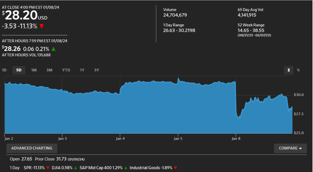
The effect of the Portland accident on Boeing’s stock price is an example of the efficiency of the stock market in processing information about a firm’s future profitability.


Glenn’s Presentation at the ASSA Session on “Making Economics Relevant: Applications of Economic Principles in the Real World”

Glenn participated in this session hosted by the National Association of Economic Educators and moderated by Kim Holder of the University of West Georgia. Glenn thanks Kim for organizing the session and for inviting him to participate.

Here is the session abstract and the list of participants:

Glenn prepared some slides for his presentation. Note that “B01″ and B02” were the titles when he first taught principles of economics as an assistant professor at Northwestern. (We won’t mention how long ago that was!)

Economists vs. the Market in Predicting the First Cut in the Federal Funds Rate

The meeting room of the FOMC in the Federal Reserve building in Washington, DC.

As we’ve noted in several recent posts, the inflation rate has fallen significantly from its peak in mid-2022, as U.S. economic growth has been slowing and the labor market appears to be less tight, slowing the growth of wages. Some economists and policymakers now believe that by early 2024, inflation will approach the Fed Reserve’s 2 percent inflation target. At that point, the Fed’s Federal Open Market Committee (FOMC) is likely to turn its attention from inflation to making sure that the U.S. economy doesn’t slip into a recession.

Accordingly, both economists and financial market participants have begun to anticipate the point at which the FOMC will begin to cut its target for the federal funds rate. (One note of caution: Fed Chair Jerome Powell has made clear that the FOMC stands ready to further increase its target for the federal funds rate if the inflation rate shows signs of increasing. He made this point most recently on December 1 in a speech at Spelman College in Atlanta.)  There is currently an interesting disagreement between economists and investors over when the FOMC is likely to cut interest rates and by how much. We can see the views of investors reflected in the futures market for federal funds.

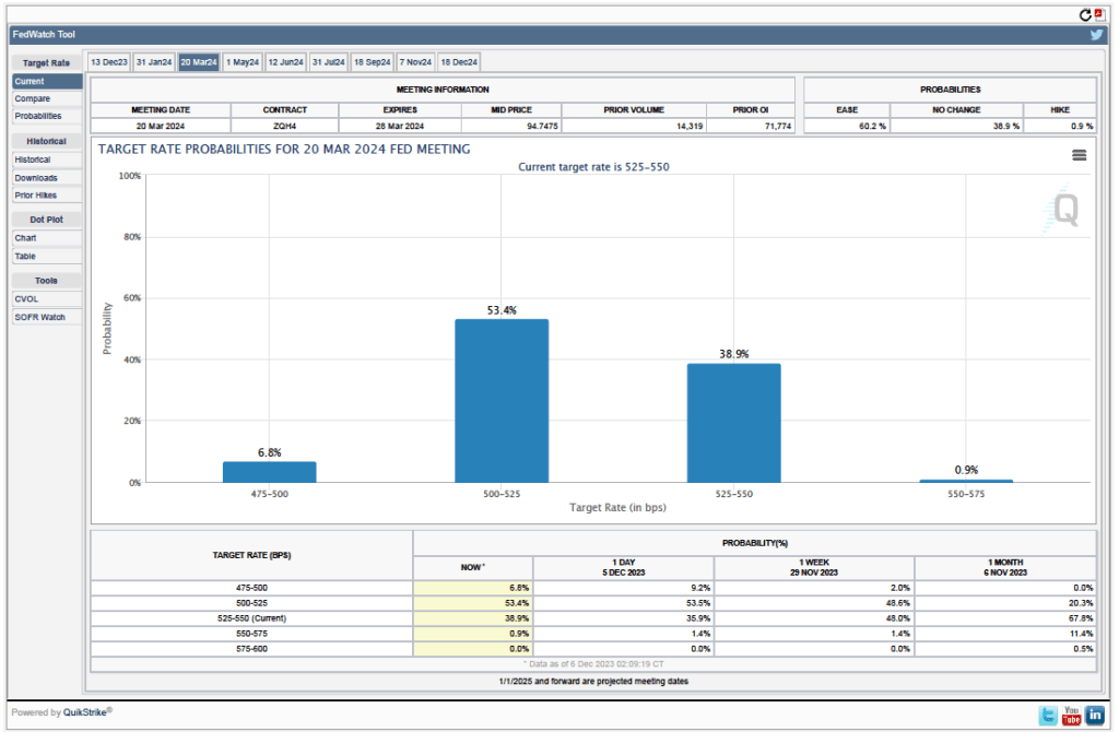
Futures markets allow investors to buy and sell futures contracts on commodities–such as wheat and oil–and on financial assets. Investors can use futures contracts both to hedge against risk—such as a sudden increase in oil prices or in interest rates—and to speculate by, in effect, betting on whether the price of a commodity or financial asset is likely to rise or fall. (We discuss the mechanics of futures markets in Chapter 7, Section 7.3 of Money, Banking, and the Financial System.) The CME Group was formed from several futures markets, including the Chicago Mercantile Exchange, and allows investors to trade federal funds futures contracts. The data that result from trading on the CME indicate what investors in financial markets expect future values of the federal funds rate to be. The following chart from the CME’s FedWatch Tool shows values after trading of federal funds futures on December 5, 2023.

The probabilities in the chart reflects investors’ predictions of what the FOMC’s target for the federal funds rate will be after the committee’s meeting on March 20, 2024. This meeting is the first after which investors currently expect that the target is likely to be lowered. The target range is currently 5.25 percent to 5.50 percent. The chart indicates that investors assign a probability of 60.2 percent to the FOMC making at least a 0.25 percentage cut in the target rate at the March meeting. 

Looking at the values for federal funds futures after the FOMC’s December 18, 2024 meeting, investors assign a 66.3 percent probability of the committee having reduced its target for the federal funds rate to 4.00 to 4.25 percent of lower. In other words, investors expect that during 2024, the FOMC will have cut its target for the federal funds rate by at least 1.25 percentage points.

Interesingly, according to a survey by the Financial Times, economists disagree with investors’ forecasts of the federal funds rate. According to the survey, which was conducted between December 1 and December 4, nearly two-thirds of economists believe that the FOMC won’t cut its target for the federal funds rate until July 2024 or later. Three-quarters of the economists surveyed believe that the FOMC will cut its target by 0.5 percent point or less during 2024. Fewer than 10 percent of the economists surveyed believe that during 2024 the FOMC will cut its target for the federal funds rate by 1.25 percent or more. (The Financial Times article describing the results of the survey can be found here. A subscription may be requred to read the article.)

So, at least among the economists surveyed by the Financial Times, the consensus is that the FOMC will cut its target for the federal funds rate later and by less than financial markets are indicating. What explains the discrepancy? The main explanation is that economists see inflation being persistently above the Fed’s 2 percent target for longer than do financial market participants. The economists surveyed are also more optimistic that the U.S. economy will avoid a recession in 2024. If a recession occurs, the FOMC is more likely to significantly cut its target than if the economy during 2024 experiences moderate growth in real GDP and the unemployment rate remains low.

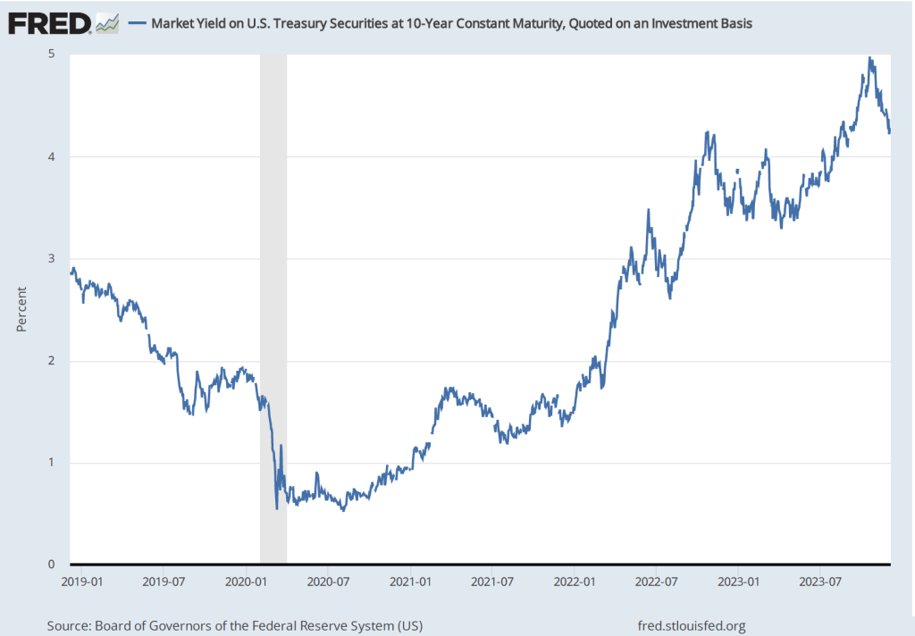
One other indication from financial markets that investors expect that the U.S. economy is likely to slow during 2024 is given by movements in the interest rate on the 10-year U.S. Treasury note. As shown in the following figure, from August to October of this year, the interest rate on the 10-year Treasury note rose from less than 4 percent to nearly 5  percent—an unusually large change in such a short period of time. Since then, most of that increase has been reversed with the interest rate on the 10-year Treasury note having fallen below 4.2 percent in early December

The movements in the interest rate on the 10-year Treasury note typically reflect investors’ expectations of future short-term interest rates. (We discuss the relationship between short-term and long-term interests rates—which economists call the term structure of interest rates—in Money, Banking, and the Financial System, Chapter 5, Section 5.2.) The increase in the 10-year interest rate between August and October reflected investors’ expectation that short-term interest rates were likely to remain persistently high for a considerable period—perhaps several years or more. The decline in the 10-year rate from late October to early December reflects investors changing their expectations toward future short-term interest rates being lower than they had previously thought. Again, as in the data on federal funds rate futures, investors seem to be expecting either slower economic growth or slower inflation than do economists.

One other complication about the interest rate on the 10-year Treasury note should be mentioned. Some of the increase in the rate from August to October may also have represented concern among investors that large federal budget deficit would cause the Treasury to issue more Treasury notes than investors would be willing to buy without the Treasury increasing the interest rate investors would receive on the newly issued notes. This concern may have been reinforced by data showing that foreign investors, particularly in China and Japan, appeared to have slowed or stopped adding to their holdings of Treasury notes. Part of the recent decline in the interest rate on the Treasury note may reflect investors becoming less concerned about these two factors.

The Roman Emperor Vespasian Fell Prey to the Lump-of-Labor Fallacy

Bust of the Roman Emperor Vespasian. (Photo from en.wikipedia.org.)

Some people worry that advances in artificial intelligence (AI), particularly the development of chatbots will permanently reduce the number of jobs available in the United States. Technological change is often disruptive, eliminating jobs and sometimes whole industries, but it also creates new industries and new jobs. For example, the development of mass-produced, low-priced automobiles in the early 1900s wiped out many jobs dependent on horse-drawn transportation, including wagon building and blacksmithing. But automobiles created many new jobs not only on automobile assembly lines, but in related industries, including repair shops and gas stations.

Over the long run, total employment in the United States has increased steadily with population growth, indicating that technological change doesn’t decrease the total amount of jobs available. As we discuss in Microeconomics, Chapter 16 (also Economics, Chapter 16), fears that firms will permanently reduce their demand for labor as they increase their use of the capital that embodies technological breakthroughs, date back at least to the late 1700s in England, when textile workers known as Luddites—after their leader Ned Ludd—smashed machinery in an attempt to save their jobs. Since that time, the term Luddite has described people who oppose firms increasing their use of machinery and other capital because they fear the increases will result in permanent job losses.

Economists believe that these fears often stem from the lump-of-labor fallacy, which holds that there is only a fixed amount of work to be performed in the economy. So the more work that machines perform, the less work that will be available for people to perform. As we’ve noted, though, machines are substitutes for labor in some uses—such as when chatbot software replace employees who currently write technical manuals or computer code—they are also complements to labor in other jobs—such as advising firms on how best to use chatbots. 

The lump-of-labor fallacy has a long history, probably because it seems like common sense to many people who see the existing jobs that a new technology destroys, without always being aware of the new jobs that the technology creates. There are historical examples of the lump-of-labor fallacy that predate even the original Luddites.

For instance, in his new book Pax: War and Peace in Rome’s Golden Age, the British historian Tom Holland (not to be confused with the actor of the same name, best known for portraying Spider-Man!), discusses an account by the ancient historian Suetonius of an event during the reign of Vespasian who was Roman emperor from 79 A.D. to 89 A.D. (p. 201):

“An engineer, so it was claimed, had invented a device that would enable columns to be transported to the summit of the [Roman] Capitol at minimal cost; but Vespasian, although intrigued by the invention, refused to employ it. His explanation was a telling one. ‘I have a duty to keep the masses fed.’”

Vespasian had fallen prey to the lump-of-labor fallacy by assuming that eliminating some of the jobs hauling construction materials would reduce the total number of jobs available in Rome. As a result, it would be harder for Roman workers to earn the income required to feed themselves.

Note that, as we discuss in Macroeconomics, Chapters 10 and 11 (also Economics, Chapter 20 and 21), over the long-run, in any economy technological change is the main source of rising incomes. Technological change increases the productivity of workers and the only way for the average worker to consume more output is for the average worker to produce more output. In other words, most economists agree that the main reason that the wages—and, therefore, the standard of living—of the average worker today are much higher than they were in the past is that workers today are much more productive because they have more and better capital to work with.

Although the Roman Empire controlled most of Southern and Western Europe, the Near East, and North Africa for more than 400 years, the living standard of the average citizen of the Empire was no higher at the end of the Empire than it had been at the beginning. Efforts by emperors such as Vespasian to stifle technological progress may be part of the reason why. 

Who Is Wealthier, Iron Man or Batman?

Photo from Paramount Pictures via britannica.com.

Photo from Warner Brothers Pictures via insider.com.

Income and wealth are often confused. Media accounts of the “wealthy” typically switch back and forth between referring to people with high incomes and referring to people with substantial wealth. It’s possible to have a high income, but not much wealth, if you spend most of your income. It’s also possible, although less common, for someone to have substantial wealth while having a relatively low income.

As we discuss in the Don’t Let This Happen to You feature in Macroeconomics, Chapter 14 (also Economics, Chapter 24), Your income is equal to your earnings during the year, while your wealth is equal to the value of the assets you own minus the value of any debts you have. It’s also worth keeping in mind that income is a flow variable that is measured over a period of time—such as a year—while wealth is a stock variable that is measured at a particular point in time—such as the first or last day of the year.

Both income and wealth can be difficult to accurately measure. Although we typically think of a person’s income as being equal to the salary and wages the person earns, income, properly measured, also includes changes in the value of the assets the person owns. For example, suppose that at the start of the year you own shares of Apple stock worth $5,000. If at the end of the year, the price on the stock market of your Apple shares has risen to $5,500, the $500 increase is part of your income for the year. (Note that this capital gain on your stock is included in your taxable income only if you sell the stock. Whether you sell the stock or not, though, the capital gain is part of your income.)

It can be difficult to measure the wealth of someone who owns significant assets that, unlike shares of stock, aren’t regularly bought and sold in a market. For instance, if someone owns a restaurant, determining what the price the restaurant would sell for—and, therefore, how wealthy the person is—can be difficult. Although other restaurants in the area may have sold recently, every restaurant is different, which makes it possible to determine only approximately what the sales price of a particular restaurant would be. As we discuss in the Apply the Concept feature “Should the Federal Government Begin to Tax Wealth?” in Microeconomics, Chapter 17 (also Economics, Chapter 17), the difficulty of valuing some types of wealth is one complication the federal government would face in enacting a tax on wealth. 

If measuring the wealth of someone in the real world is difficult, measuring the wealth of a fictional character is even more daunting. Some years ago, undergraduate students, most of whom were economics majors at Lehigh University, estimated the wealth of Bruce Wayne, the alter ego of Batman. To narrow the focus, the students based their estimate on only the information available in the three Batman films directed by Christopher Nolan. On the basis of that information, they estimate that Bruce Wayne’s wealth is $11.6 billion. At the time the films were produced, that would have made Bruce Wayne the seventy-third wealthiest person in the world—if, of course, he had been a real person! You can read the details of their estimate here. 

Bruce Wayne is apparently very wealthy, but is he as wealthy as Tony Stark, the alter ego of Iron Man? Apparently not, according to an estimate appearing on the business web site forbes.com. Although he doesn’t seem to give the details of how he arrived at the estimate, the author of the post values Tony Stark’s wealth at $9.3 billion, making him about 20 percent less wealthy than Bruce Wayne.  Score one for the Caped Crusader!

California Deals with the Paradox of Tobacco Taxes

(Photo from Zuma Press via the Wall Street Journal.)

When state and local governments impose taxes on sales of liquor, on cigarettes and other tobacco products, or on soda and other sweetened beverages, they typically have two objectives: (1) Discourage consumption of the taxed goods, and (2) raise revenue to pay for government services.  As we discuss in Chapter 6 of Microeconomics (also Economics, Chapter 6), these objectives can be at odds with each other. The tax revenue a government receives depends on both the size of the tax and the number of units sold. Therefore, the more successful a tax is in significantly reducing, say, sales of cigarettes, the less tax revenue the government receives from the tax.

As we discuss in Chapter 6, a tax on a good shifts the supply curve for the good up by the amount of the tax. (We think it’s intuitively easier to think of a tax as shifting up a supply curve, but analytically the effect on equilibrium is the same if we illustrate the effect of the tax by shifting down the demand curve for the taxed good by the amount of the tax.)  A tax will raise the equilibrium price consumers pay and reduce the equilibrium quantity of the taxed good that they buy. For a supply curve of a given price elasticity in the relevant range of prices, how much a tax increases equilibrium  price relative to how much it decreases equilibrium quantity is determined by the price elasticity of demand. 

The following figure illustrates these points. If a city implements a tax of $0.75 per 2-liter bottle of soda, the supply curve shifts up from S1 to S2. If demand is price elastic, the equilibrium price increases from $1.75 to $2.00, while the equilibrium quantity falls from 90,000 bottles per day to 70,000. If demand is price inelastic, the equilibrium price rises by more, but the equilibrium quantity falls by less. Therefore, a more price elastic demand curve is good news for objective (1) above—soda consumption falls by more—but bad news for the amount of tax revenue the government collects. When the demand for soda is price inelastic, the government collects tax revenue of $0.75 per bottle multiplied by 80,000 bottles, or $60,000 per day. When the demand for soda is price elastic, the government collects tax revenue of $0.75 per bottle multiplied by 70,000 bottles, or only $52,500 per day.

One further point: We would expect the amount of revenue the government earns from the tax to decline over time, holding constant other variables that might affect the market for the taxed good, . This conclusion follows from the fact that demand typically becomes more price elastic over time. In other words, when a tax is first imposed (or an existing tax is increased), consumers are likely to reduce purchases of the taxed good less in the short run than in the long run. This result can a problem for governments that make a commitment to use the tax revenues for a particular purpose.

A recent article in the Los Angeles Times highlighted this last point. In 1999, California voters passed Proposition 10, which increased the tax on cigarettes by $0.50 per pack, with similar tax increases on other tobacco products. The tax revenues were dedicated to funding “First 5” state government agencies, which are focused on providing services to children 5 years old and younger.  The article notes, as the above analysis would lead us to expect, that the additional revenue the state received from the tax increase was largest in the first year and has gradually declined since as the quantity of cigarettes and other tobacco products sold has fallen. (Note that over such a long period of time, other factors in addition to the effects of the tax have contributed to the decline in smoking in California.) As a result, the state and county governments have had to scramble to find additional sources of funds for the First 5 agencies. The article quotes Deborah Daro, a researcher at the University of Chicago, as noting: “It seemed like a brilliant solution—tax the sinners who are smoking to help newborns and their parents …. But then people stopped smoking, which from a public health perspective is great, but from a funding perspective for First 5—they don’t have another funding stream.”

Claudia Goldin Wins the Nobel Prize in Economics

Claudia Goldin (Photo from Goldin’s web page at havard.edu.)

Claudia Goldin, the Henry Lee Professor of Economics at Harvard, has been awarded the 2023 Nobel Prize in Economic Sciences. Goldin’s research is wide-ranging, with a focus on the economic history of women and on gender disparities in wages and employment. She received her PhD from the University of Chicago in 1972 for a thesis that was published in 1976 as Urban Slavery in the American South, 1820 to 1860: A Quantitative History. Her thesis adviser, Robert Fogel, was awarded the Nobel Prize in 1993 for his work in economic history. He shared the prize that year with Douglas North of Washington University in St. Louis. Goldin’s work on economic history contributed to the cliometric revolution, which involves the application of theoretical models and econometric methods to the study of historical issues.  At the time of the award to Fogel and North, Goldin discussed their research and the cliometric revolution here.

Goldin’s pioneering and influential research on the economic history of women was the basis for her 1990 book Understanding the Gender Gap: An Economic History of American Women. The themes of that book were expanded on in 2021 in Career & Family: Women’s Century-Long Journey toward Equity, and in her forthcoming An Evolving Force: A History of Women in the Economy.

In research with Lawrence Katz, also a professor of economics at Harvard, Goldin has explored how technological change and educational attainment have affected income inequality, particularly the wage premium skilled workers receive. Goldin and Katz summarized their findings in 2008 in the influential book, The Race between Education and Technology.

The wide scope of Goldin’s research can be seen by reviewing her curriculum vitae, which can be found here. The announcement by the Nobel committee can be found here.

9/16/23 Podcast – Authors Glenn Hubbard & Tony O’Brien discuss inflation, the current status of a soft-landing, and the green economy.

Join authors Glenn Hubbard & Tony O’Brien as they discuss the economic landscape of inflation, soft-landings, and the green economy. This conversation occurred on Saturday, 9/16/23, prior to the FOMC meeting on September 19th-20th.

A Reporter for NPR Encounters the Challenge of Network Externalities on an EV Road Trip

An electric vehicle (EV) charging station. (Photo from the Associated Press via the Wall Street Journal.)

Secretary of Energy Jennifer Granholm recently took a road trip in a caravan of electric vehicles (EVs). The road trip “was intended to draw attention to the billions of dollars the White House is pouring into green energy and clean cars.” A reporter for National Public Radio (NPR) went on the trip and wrote an article on her experience.

One conclusion the reporter drew was: “Riding along with Granholm, I came away with a major takeaway: EVs that aren’t Teslas have a road trip problem, and the White House knows it’s urgent to solve this issue.” The problem was that charging stations are less available and less likely to be functioning than would be needed for a road trip in an EV to be as smooth as a similar trip in a gasoline-powered car. The reporter noted that in her experience with her own EV: “I use multiple apps to find chargers, read reviews to make sure they work and plot out convenient locations for a 30-minute pit stop (a charger by a restaurant, for instance, instead of one located at a car dealership).”

EVs exhibit network externalities. As we discuss in Microeconomics and Economics, Chapter 10, 10.3 (Essentials of Economics, Chapter 7, Section 7.3), Network externalities are a situation in which the usefulness of a product increases with the number of consumers who use it. For example, the more iPhones people buy, the more profit firms and individuals can earn by creating apps for the iPhone. And the more apps that are available, the more useful an iPhone becomes to people who use it.

In this blog post, we discuss how Mark Zuckerberg’s Meta Platforms (which was originally named Facebook) has had difficulty selling Oculus augmented reality headsets. Many people have been reluctant to buy these headsets because they don’t believe there are enough software programs available to use the headsets with. Software designers don’t have much incentive to produce such programs because not many consumers own a headset necessary to use the programs.

The difficulty that Meta has experienced with augmented reality headsets can be overcome if the product is sufficiently useful that consumers are willing to buy it even if complementary products are not yet available. That was the case with the iPhone, which experienced strong sales even before Apple opened its app store. Or to take an historical example relevant to the current situation with EVs: When the Ford Motor Company introduced the Model T car in the early twentieth century, many people found that owning a car was such an advance over using a horse-drawn vehicle that they were willing to buy one despite there being realtively few gas stations and repair shops available. Because so many cars were being sold, entrepreneurs had an incentive to begin opening gas stations and repair shops, which increased the attractiveness of using a car, thereby further increasing demand.

As the NPR reporter’s experience shows, consumers choosing between buying an EV or a gasoline-powered car are in a situation similar to that faced by early twentieth century consumers in choosing between cars and horse-drawn vehicles. One difference between the two situations is that Congress and the Biden administration are attempting to ease the transition to EVs by subsidizing the construction of charging stations and by providing tax credits to people who buy EVs.

Solved Problem: The German Tobacco Tax and Price Elasticity

(Photo from Reuters via the Wall Street Journal)

Supports: Microeconomics, Chapter 6, Section 6.3, Economics, Chapter 6, Section 6.3, and Essentials of Economics, Chapter 7, Section 7.7.

In August 2023, an article in the Wall Street Journal discussed the effort of the German government to reduce tobacco use. As part of the effort, the government increased the tax on tobacco products, including cigars and cigarettes. The tax increase took effect on January 1, 2022. According to German government data, during 2022 the quantity of cigars and cigarettes sold declined by 8.3 percent. At the same time, the tax revenue the government collected from the tobacco tax declined from €14.7 billion to €14.2 billion.

  1. From this information, can you determine whether the tobacco tax raised the price of cigars and cigarettes by more or less than 8.3 percent? Can you determine whether the demand for cigars and cigarettes in Germany is price elastic or price inelastic? Briefly explain.
  2. According to the Wall Street Journal article, in addition to increasing the tax on tobacco products, the German government took other steps, including banning outdoor advertising of tobacco products, to discourage smoking. Does this additional information affect your answer to parts a.? Briefly explain. 

Solving the Problem

Step 1:  Review the chapter material. This problem is about the effect of price changes on revenue, so you may want to review Microeconomics, Chapter 6, Section 6.3, “The Relationship between Price Elasticity of Demand and Total Revenue,” or the corresponding sections in Economics, Chapter 6 or Essentials of Economics, Chapter 7.

Step 2: Answer part a. by explaining whether you can tell if the tobacco tax raised the price of cigars and cigarettes by more than 8.3 percent and whether the demand for cigars and cigarettes in Germany is price elastic or price inelastic. We have two pieces of information: (1) In 2022, the quantity of cigars and cigarettes sold in Germany fell by 8.3 percent, and (2) the revenue the German government collected from the tobacco tax fell. We know that if a company increases the price of its product and the total revenue it earns falls, then the demand for the product must be price elastic. We can apply that same reasoning to a government increasing a tax. If the tax increase leads to a fall in revenue we can conclude that the demand for the good being taxed (in this case cigars and cigarettes) is price elastic.  When the demand for a good is price elastic, the percentage change in the quantity demanded resulting from a price increase will be greater than the percentage change in the price.  Therefore, the percentage change in price resulting from the tax must be less than 8.3 percent. An important qualification to this conclusion is that it holds only if no variable, other than the increase in the tax, affected the demand for cigars and cigarettes during 2022.

Step 3: Answer part b. by explaining how the German government’s banning of outdoor advertising of tobacco products affects your answer to part a. Banning outdoor advertising of tobacco products may have reduced the demand for cigars and cigarettes. If the demand curve for cigars and cigarettes shifted to left, then some of the 8.3 percent decline in the quantity sold may have been the result of the shift in demand rather than the result of the increase in the tax. In other words, the German market for cigars and cigarettes in 2022 may have experienced both a decrease in demand—as the demand curve shifted to the left—and a decrease in the quantity demanded—as the tax increase raised the price of cigars and cigarettes. Given this new information, we can’t be sure that our conclusions in part a.—that the demand for cigars and cigarettes is price elastic and that the tax resulted in an increase in the price of less than 8.3 percent—are correct.  

Extra credit:  This discussion indicates that in practice economists have to use statistical methods when they estimate the price elasticity of demand for a good or service. The statistical methods make it possible to distinguish the effect of a movement along a demand curve as the price changes from a shift in the demand curve caused by changes in other economic variables.  

Sources:  Jimmy Vielkind, “Smoking Is a Dying Habit. Not in Germany,” Wall Street Journal, August 31, 2023; and Statistisches Bundesamt, “Taxation of Tobacco Products (Cigarettes, Cigars/Cigarillos, Fine-Cut Tobacco, Pipe Tobacco): Germany, Years, Tax Stamps,” September 10, 2023.