Figure from CBO’s monthly budget report.
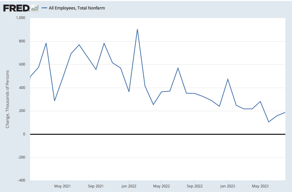
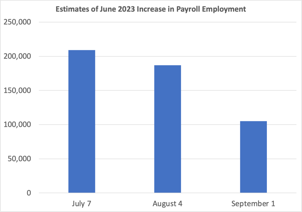
During 2023, GDP and employment have continued to expand. Between the second quarter of 2022 and the second quarter of 2023, nominal GDP increased by 6.1 percent. From July 2022 to July 2023, total employment increased by 3.3 million as measured by the establishment (or payroll) survey and by 3.0 as measured by the household survey. (In this post, we discuss the differences between the employment measures in the two surveys.)
We would expect that with an expanding economy, federal tax revenues would rise and federal expenditures on unemployment insurance and other transfer programs would decline, reducing the federal budget deficit. (We discuss the effects of the business cycle on the federal budget deficit in Macroeconomics, Chapter 16, Section 16.6, Economics, Chapter 26, Section 26.6, and Essentials of Economics, Chapter 18, Section 18.6.) In fact, though, as the figure from the Congressional Budget Office (CBO) at the top of this post shows, the federal budget deficit actually increased substantially during 2023 in comparison with 2022. The federal budget deficit from the beginning of government’s fiscal year on October 1, 2022 through July 2023 was $1,617 billion, more than double the $726 billion deficit during the same period in fiscal 2022.
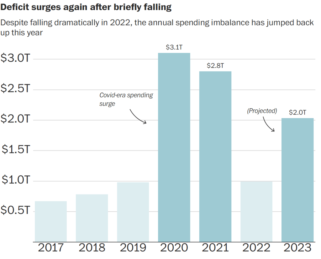
The following figure from an article in the Washington Post uses data from the Committee for a Responsible Federal Budget to illustrate changes in the federal budget deficit in recent years. The figure shows the sharp decline in the federal budget deficit in 2022 as the economic recovery from the Covid–19 pandemic increased federal tax receipts and reduced federal expenditures as emergency spending programs ended. Given the continuing economic recovery, the surge in the deficit during 2023 was unexpected.
As the following figure shows, using CBO data, federal receipts—mainly taxes—are 10 percent lower this year than last year, and federal outlays—including transfer payments—are 11 percent higher. For receipts to fall and outlays to increase during an economic expansion is very unusual. As an article in the Wall Street Journal put it: “Something strange is happening with the federal budget this year.”
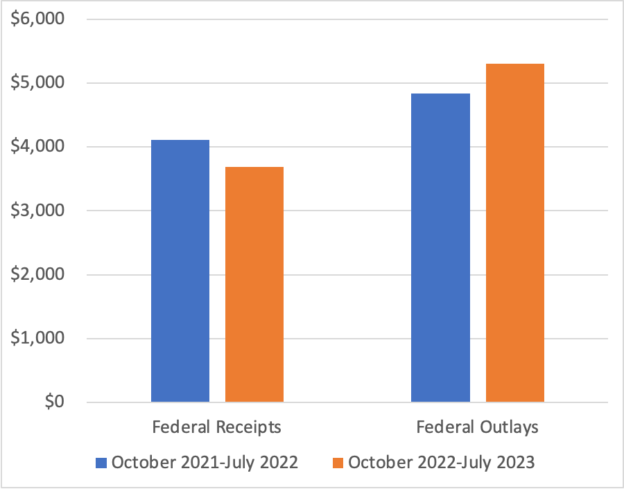
Note: The values on the vertical axis are in billions of dollars.
The following figure shows a breakdown of the decline in federal receipts. While corporate taxes and payroll taxes (primarily used to fund the Social Security and Medicare systems) increased, personal income tax receipts fell by 20 percent, and “other receipts” fell by 37 percent. The decline in other receipts is largely the result of a decline in payments from the Federal Reserve to the U.S. Treasury from $99 billion in 2022 to $1 billion in 2023. As we discuss in Macroeconomics, Chapter 17, Section 17.4 (Economics, Chapter 27, Section 27.4), Congress intended the Federal Reserve to be independent of the rest of the government. Unlike other federal agencies and departments, the Fed is self-financing rather than being financed by Congressional appropriations. Typically, the Fed makes a profit because the interest it earns on its holdings of Treasury securities is more than the interest it pays banks on their reserve deposits. After paying its operating costs, the Fed pays the rest of its profit to the Treasury. But as the Fed increased its target for the federal funds rate beginning in March 2022, it also increased the interest rate it pays banks on their reserve deposits. Because most of the securities it holds pay low interest rates, the Fed has begun running a deficit, reducing the payments it makes to the Treasury.
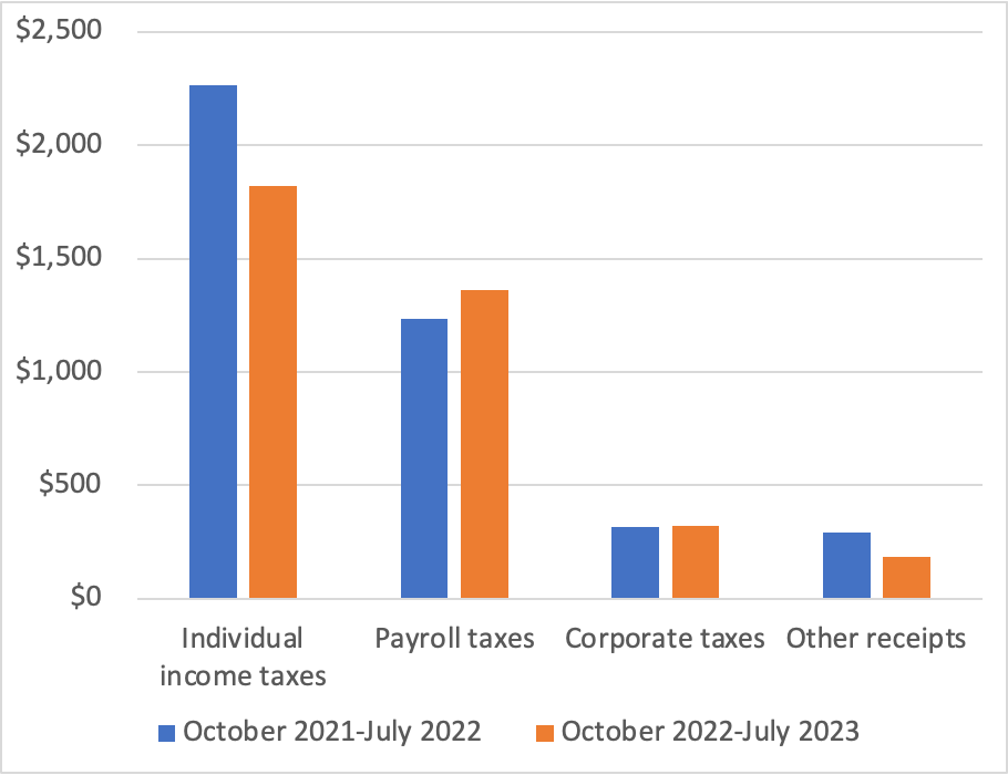
Note: The values on the vertical axis are in billions of dollars.
The reasons for the sharp decline in individual income taxes are less clear. The decline was in the “nonwithheld category” of individual income taxes; federal income taxes withheld from worker paychecks increased. People who are self-employed or who receive substantial income from sources such as capital gains from selling stocks, make quarterly estimated income tax payments. It’s these types of personal income taxes that have been unexpectedly low. Accordingly, smaller capital gains may be one explanation for the shortfall in federal revenues, but a more complete explanation won’t be possible until more data become available later in the year.
The following figure shows the categories of federal outlays that have increased the most from 2022 to 2023. The largest increase is in spending on Social Security, Medicare, and Medicaid, with spending on Social Security alone increasing by $111 billion. This increase is due partly to an increase in the number of retired workers receiving benefits and partly to the sharp rise in inflation, because Social Security is indexed to changes in the consumer price index (CPI). Spending on Medicare increased by $66 billion or a surprisingly large 18 percent. Interest payments on the public debt (also called the federal government debt or the national debt) increased by $146 billion or 34 percent because interest rates on newly issued Treasury securities rose as nominal interest rates adjusted to the increase in inflation and because the public debt had increased significantly as a result of the large budget deficits of 2020 and 2021. The increase in spending by the Department of Education reflects the effects of the changes the Biden administration made to student loans eligible for the income-driven repayment plan. (We discuss the income-driven repayment plan for student loans in this blog post.)
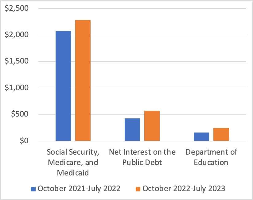
Note: The values on the vertical axis are in billions of dollars.
The surge in federal government outlays occurred despite a $120 billion decline in refundable tax credits, largely due to the expiration of the expansion of the child tax credit Congress enacted during the pandemic, a $98 billion decline in Treasury payments to state and local governments to help offset the financial effects of the pandemic, and $59 billion decline in federal payments to hospitals and other medical facilities to offset increased costs due to the pandemic.
In this blog post from February, we discussed the challenges posed to Congress and the president by the CBO’s forecasts of rising federal budget deficits and corresponding increases in the federal government’s debt. The unexpected expansion in the size of the federal budget deficit for the current fiscal year significantly adds to the task of putting the federal government’s finances on a sound basis.