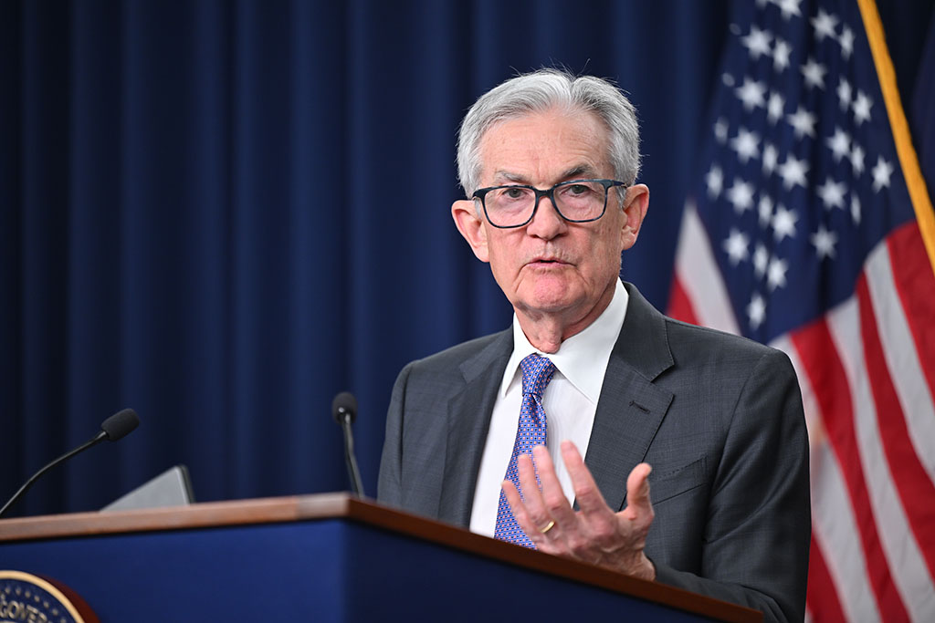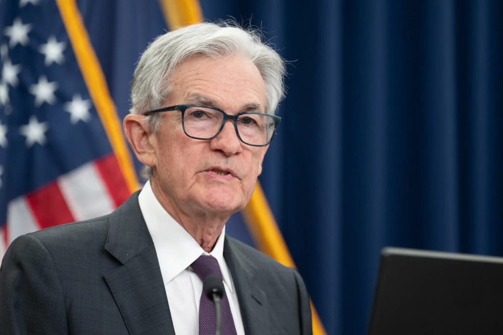
Photo from federalreserve.gov
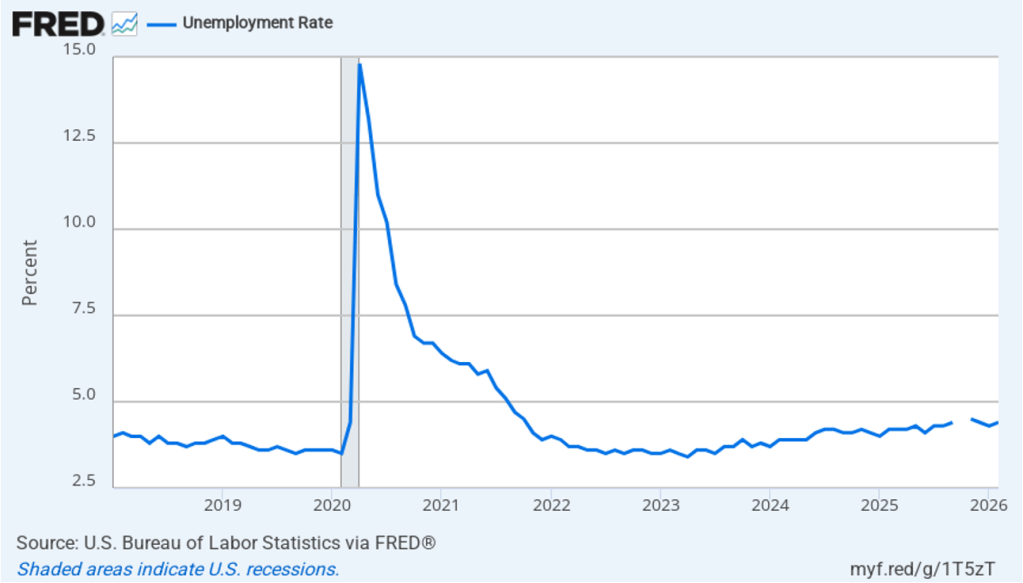
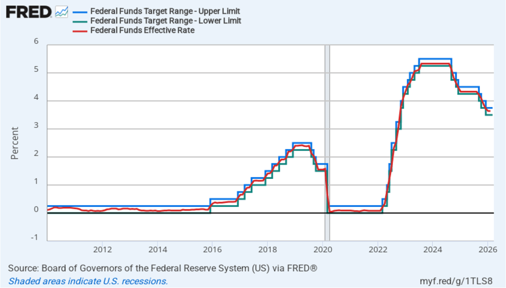
Today’s meeting of the Federal Reserve’s policymaking Federal Open Market Committee (FOMC) had the expected result with the committee deciding to leave unchanged its target for the federal funds rate at its current range of 3.50 percent to 3.75 percent. The members of the committee voted 11 to in favor of the decision. Fed Governor Stephen Miran voted against the decision, preferring to lower the target range for the federal funds rate by 0.25 percentage point (25 basis points).
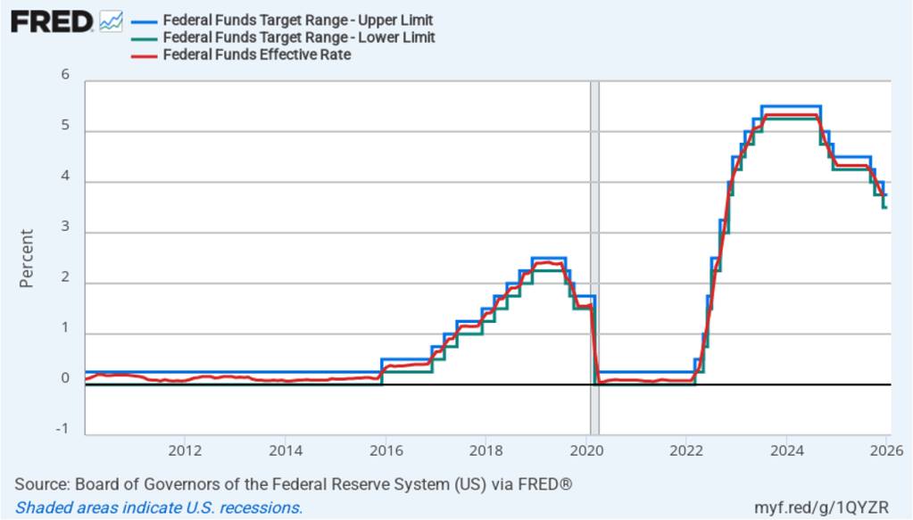
The following figure shows for the period since January 2010, the upper bound (the blue line) and the lower bound (the green line) for the FOMC’s target range for the federal funds rate, as well as the actual values for the federal funds rate (the red line). Note that the Fed has been successful in keeping the value of the federal funds rate in its target range. (We discuss the monetary policy tools the FOMC uses to maintain the federal funds rate within its target range in Macroeconomics, Chapter 15, Section 15.2 (Economics, Chapter 25, Section 25.2).)
After the meeting, the committee also released a “Summary of Economic Projections” (SEP)—as it typically does after its March, June, September, and December meetings. The SEP presents median values of the 19 committee members’ forecasts of key economic variables. The values are summarized in the following table, reproduced from the release. (Note that only 5 of the district bank presidents vote at FOMC meetings, although all 12 presidents participate in the discussions and prepare forecasts for the SEP.)
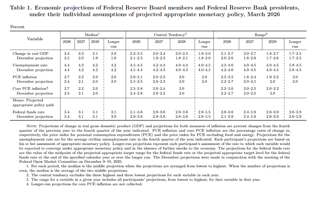
There are several aspects of these forecasts worth noting:
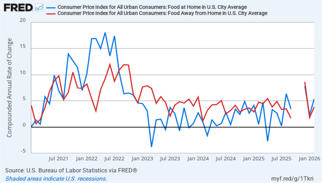
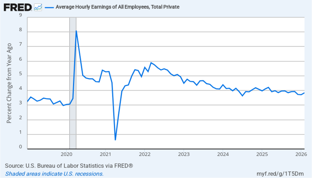
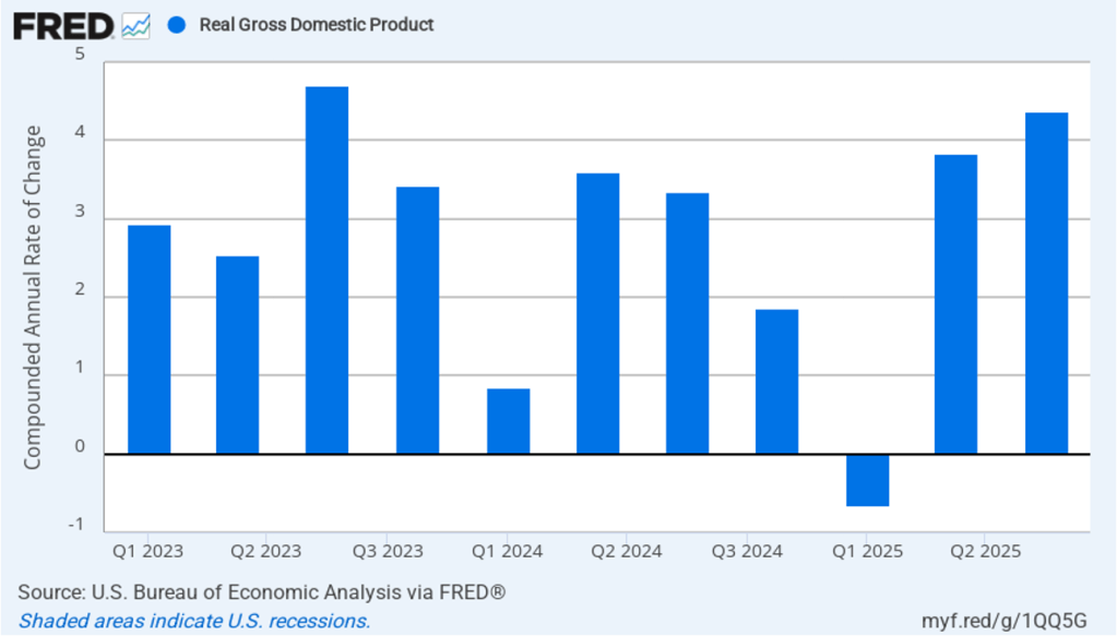
- Compared with December, the committee members increased their forecasts of real GDP growth for each year from 2025 through 2027. The committee members also increased their forecast of long-run growth in real GDP to 2.0 percent from 1.8 percent in December. Although that increase may seem small, as we discuss in Macroeconomics, Chapter 10, Section 10.1 (Economics, Chapter 20, Section 20.1), over time, small increases in growth rates in real GDP can result in substantial increases in the standard of living. Despite increasing their forecast of growth in real GDP, committee members left their forecasts of the unemployment rate unchanged.
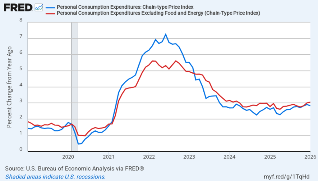
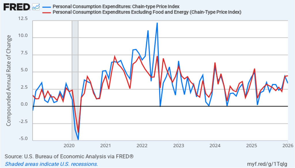
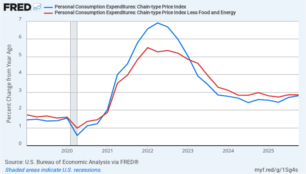
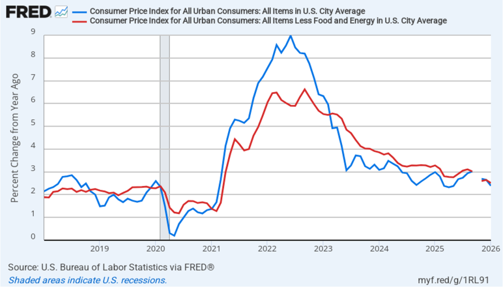
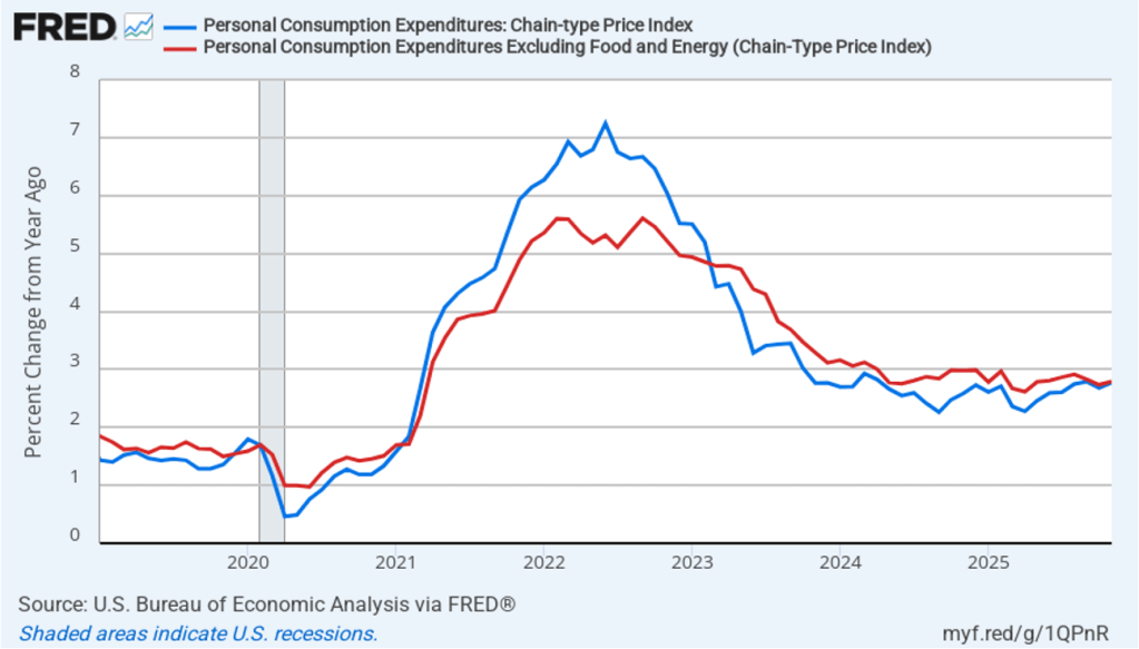
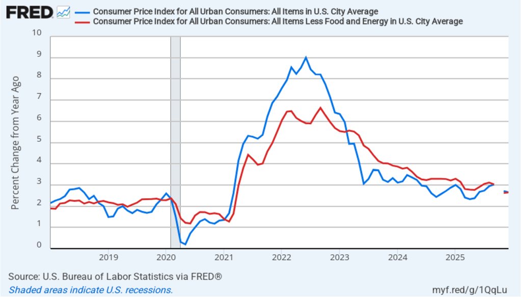
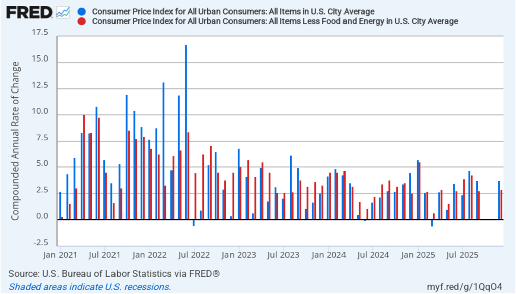
- Committee members reduced their forecast for 2026 of personal consumption expenditures (PCE) price inflation significantly to 2.7 percent from 2.4 percent in December. They raised their forecast for inflation in 2027 slightly and continued to forecast that PCE inflation will decline to the Fed’s 2.0 percent annual target in 2028.
- The committee’s forecasts of the federal funds rate at the end of each year from 2026 through 2028 were unchanged but the forecast for the long-run federal funds rate was increased to 3.1 percent from 3.0 percent in December.
Prior to the meeting there was much discussion in the business press and among investment analysts about the dot plot, shown below. Each dot in the plot represents the projection of an individual committee member. (The committee doesn’t disclose which member is associated with which dot.) Note that there are 19 dots, representing the 7 members of the Fed’s Board of Governors and all 12 presidents of the Fed’s district banks.
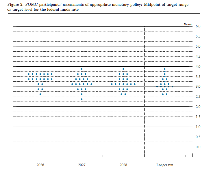
The plots on the far left of the figure represent the projections by the 19 members of the value of the federal funds rate at the end of 2026. The plots indicate that at this point there is majority support on the committee for one 25 basis point cut by the end of the year in the federal funds rate from its current range of 3.50 percent to 3.25 percent to a range of 3.25 percent to 3.00 percent. The plots on the far right of the figure indicate that there is substantial disagreement among committee members as to what the long-run value of the federal funds rate—the so-called neutral rate—should be. Of course, the plots only represent the forecasts of the committee members and individual committee members are likely to adjust their forecasts as additional macroeconomic data become available in the coming months.
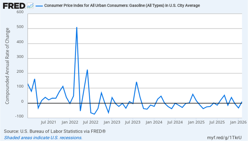
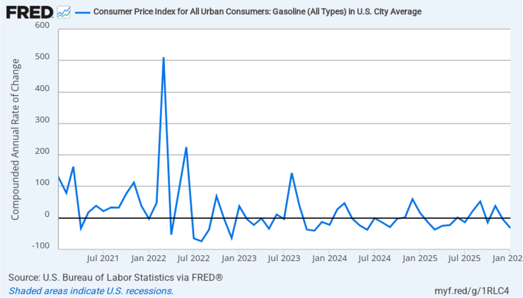
During his press conference following the meeting, Powell indicated that the effects of the conflict in Iran on the U.S. economy were uncertain. He noted that traditionally central banks “look through” increases in oil prices because they result in only a one-time increase in the price level rather than in sustained inflation. He noted, though, that the committee might take steps to offset the effect of higher oil prices if there were an indication that the price increases were affecting long-run expectations of inflation.
He noted that the increase in inflation in recent months was largely due to the effects of the increase in tariffs on goods prices. Powell indicated that committee members expect that the tariff increases will have largely passed through the economy by the middle of the year. Powell attributed committee members increasing their forecast of long-run growth in real GDP to their expectation that recent increases in productivity growth would be sustained.
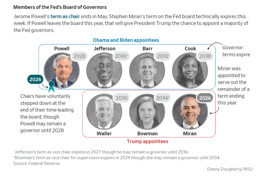
Finally, Powell discussed the end of his term as chair on May 15. (Powell will be chair for one more meeting of the FOMC on April 28–29.) He stated that if the Senate doesn’t confirm Kevin Warsh as his replacement as chair by May 15, he would follow the law and Fed tradition by continuing to serve as chair in a temporary capacity. Powell’s term as a member of the Board of Governors doesn’t end until January 31, 2028. He indicated that he will only step down from his position on the Board if the legal case the Department of Justice has opened against him for having given allegedly false testimony to Congress is “well and truly over, with transparency and finality.”