Image created by ChatGPT
There has been an ongoing debate about whether Millennials and people in Generation Z are better off or worse off economically than are Baby Boomers. Edward Wolff of New York University recently published a National Bureau of Economic Research (NBER) working paper that focuses on one aspect of this debate—how the wealth of households headed by someone 75 years and older changed relative to the wealth of households headed by someone 35 years and younger during the period from 1983 to 2022.
Wolff uses data from the Federal Reserve’s Survey of Consumer Finances to measure the wealth, or net worth, of people in these age groups—the market value of their financial assets minus the market value of their financial liabilities. He includes in his measure of assets the market value of people’s real estate holdings—including their homes—stocks and bonds, bank deposits, contributions to defined contribution pension funds, unincorporated businesses, and trust funds. He includes in his measure of liabilities people’s mortgage debt, consumer debt—including credit card balances—and other debt, such as educational loans. Because Wolff wants to focus on that part of wealth that is available to be spent on consumption, he refers to it as financial resources, and he excludes from his wealth measure the present value of future Social Security payments and the present value of future defined contribution pension benefits.
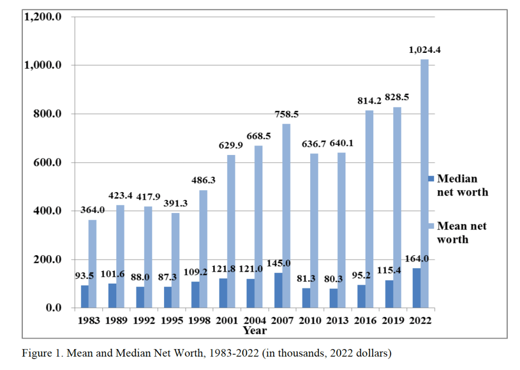
The following figure from Wolff’s paper shows that, using his definition, both median and mean wealth have increased substantially from 1987 to 2o22. Note that both measures of average wealth declined during the Great Recession and Global Financial Crisis of 2007–2009. Median wealth declined by nearly 44 percent between 2007 and 2010. That median wealth grew much faster than mean wealth over the whole period indicates that wealth inequality.
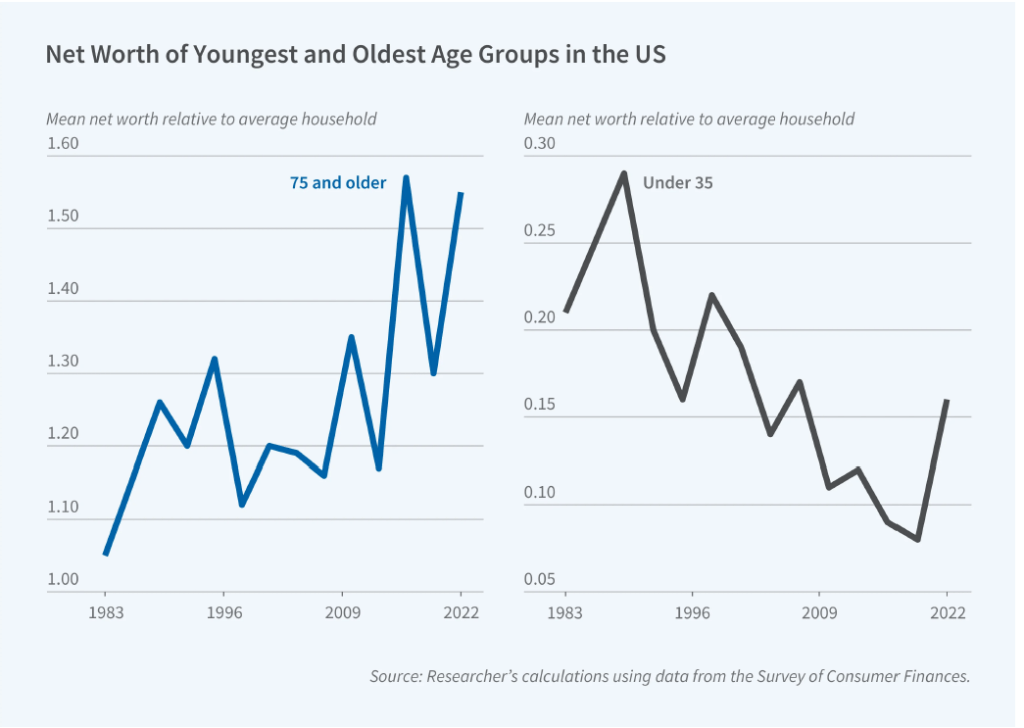
Although the average wealth of all age groups increased over this period, the relative wealth of households 75 years and older rose and the relative wealth of households 35 years and younger fell. The following figure from the NBER Digest illustrates this shift. The 75 and over age group increased its mean net worth from 5 percent greater than the mean net worth of the average household in 1983 to 55 percent of the mean net worth of the average household in 2022. In contrast, the 35 and under age group saw its mean new worth relative to the average household fall from 21 percent in 1983 to 16 percent in 2022. Note, though, that there is significant volatility over time in the relative wealth shares of the two age groups.
What explains the relative increase in wealth among households 75 and over and the relative decrease in wealth among households 35 and under? Wolff identifies three key factors:
“[T]he homeownership rate, total stocks directly and indirectly owned, and home mortgage debt. The homeownership rate is the same in the two years for the youngest group but falls relative to the overall rate, whereas it shoots up for the oldest group both in actual level and relative to the overall average. The value of stock holdings rises for both age groups but vastly more for the oldest households compared to the youngest ones and accounts for a substantial portion of the elderly’s relative wealth gains. Mortgage debt rises in dollar terms for both groups but considerably more in relative terms for the youngest group.”
Perhaps surprisingly, Wolff finds that “despite dire press reports, educational loans fail to appear as a significant factor” in explaining the decline in the relative wealth of younger households.