Has AI Damaged the Tech Job Market for Recent College Grads?

Image generated by ChatGPT 5

“Artificial intelligence is profoundly limiting some young Americans’ employment prospects, new research shows.” That’s the opening sentence of a recent opinion column in the Wall Street Journal. The columnist was reacting to a new academic paper by economists Erik Brynjolfsson, Bharat Chandar, and Ruyu Chen of Stanford University. (See also this Substack post by Chandar that summarizes the results of their paper.) The authors find that:

“[S]ince the widespread adoption of generative AI, early-career workers (ages 22-25) in the most AI-exposed occupations have experienced a 13 percent relative decline in employment … In contrast, employment for workers in less exposed fields and more experienced workers in the same occupations has remained stable or continued to grow. Furthermore, employment declines are concentrated in occupations where AI is more likely to automate, rather than augment, human labor.”

The authors conclude that “our results are consistent with the hypothesis that generative AI has begun to significantly affect entry-level employment.”

About a month ago, we wrote a blog post looking at whether unemployment among young college graduates has been abnormally high in recent months.  The following figure from that post shows that over time, the unemployment rates for the youngest college graduates (the red line) is nearly always above the unemployment rate for the population as a whole (the green line), while the unemployment rate for college graduates 25 to 34 years old (the blue line) is nearly always below the unemployment rate for the population as a whole. In July of this year, the unemployment rate for the population as a whole was 4.2 percent, while the unemployment for college graduates 20 to 24 years old was 8.5 percent, and the unemployment rate for college graduates 25 to 34 years old was 3.8 percent.

As the following figure (also reproduced from that blog post) shows, the increase in unemployment among young college graduates has been concentrated among males. Does higher male unemployment indicate that AI is eliminating jobs, such as software coding, that are disproportionately male? Data journalist John Burn-Murdoch argues against this conclusion, noting that data shows that “early-career coding employment is now tracking ahead of the [U.S.] economy.”

Another recent paper written by Sarah Eckhardt and Nathan Goldschlag of the Economic Innovation Group is also skeptical of the view that firms adopting generative AI programs is reducing employment in certain types of jobs. They use a measure developed by Edward Felton on Princeton University, and Manav Raj and Robert Seamans of New York University of how exposed particular jobs are to AI (AI Occupational Exposure (AIOE)). The following table from Eckhardt and Goldschlag’s paper shows the five most AI exposed jobs and the five least AI exposed jobs.

They divide all occupations into quintiles based on the exposure of the occupations to AI. Their key results are given in the following table, which shows that the occupations that are most exposed to the effects of AI—quintiles 4 and 5—have lower unemployment rates and higher wages than do the occupations that are least exposed to AI. 

The Brynjolfsson, Chandar, and Chen paper mentioned at the beginning of this post uses a larger data set of workers by occupation from ADP, a private firm that processes payroll data for about 25 percent of U.S. workers. Figure 1 from their paper, reproduced here, shows that employment of workers in two occupations—software developers and customer service—representative of those occupations most exposted to AI declined sharply after generative AI programs became widely available in late 2022.

They don’t find this pattern for all occupations, as shown in the following figure from their paper.

Finally, they show results by occupational quintiles, with workers ages aged 22 to 25 being hard hit in the two occupational quintiles (4 and 5) most exposted to AI. The data show total employment growth from October 2022 to July 2025 by age group and exposure to AI.

Economics blogger Noah Smith has raised an interesting issue about Brynjolfsson, Chandar, and Chen’s results. Why would we expect that the negative effect of AI on employment to be so highly concentrated among younger workers? Why would employment in the most AI exposed occupations be growing rapidly among workers aged 35 and above? Smith wonders “why companies would be rushing to hire new 40-year-old workers in those AI-exposed occupations.” He continues:

“Think about it. Suppose you’re a manager at a software company, and you realize that the coming of AI coding tools means that you don’t need as many software engineers. Yes, you would probably decide to hire fewer 22-year-old engineers. But would you run out and hire a ton of new 40-year-old engineers?

Both the papers discussed here are worth reading for their insights on how the labor market is evolving in the generative AI era. But taken together, they indicate that it is probably too early to arrive at firm conclusions about the effects of generative AI on the job market for young college graduates or other groups.

Glenn’s Questions for the Fed

Photo from federalreserve.gov

This opinion column originally ran at Project Syndicate.

While recent media coverage of the US Federal Reserve has tended to focus on when, and by how much, interest rates will be cut, larger issues loom. The selection of a new Fed chair to succeed Jerome Powell, whose term ends next May, should focus not on short-term market considerations, but on policies and processes that could improve the Fed’s overall performance and accountability.

By demanding that the Fed cut the federal funds rate sharply to boost economic activity and lower the government’s borrowing costs, US President Donald Trump risks pushing the central bank toward an overly inflationary monetary policy. And that, in turn, risks increasing the term premium in the ten-year Treasury yield—the very financial indicator that Treasury Secretary Scott Bessent has emphasized. A higher premium would raise, not lower, borrowing costs for the federal government, households, and businesses alike. Moreover, concerns about the Fed’s independence in setting monetary policy could undermine confidence in US financial markets and further weaken the dollar’s exchange rate. 

But this does not imply that Trump should simply seek continuity at the Fed. The Fed, under Powell, has indeed made mistakes, leading to higher inflation, sometimes inept and uncoordinated communications, and an unclear strategy for monetary policy.

I do not share the opinion of Trump and his advisers that the Fed has acted from political or partisan motives. Even when I have disagreed with Fed officials or Powell on matters of policy, I have not doubted their integrity. However, given their mistakes, I do believe that some institutional introspection is warranted. The next chair—along with the Board of Governors and the Federal Open Market Committee—will have many policy questions to address beyond the near-term path for the federal funds rate. 

Three issues are particularly important. The first is the Fed’s dual mandate: to ensure stable prices and maximum employment. Many economists (including me) have been critical of the Fed for exhibiting an inflationary bias in 2021 and 2022. The highest inflation rate in 40 years raised pressing questions about whether the Fed has assigned the right weights to inflation and employment. 

Clearly, the strategy of pursuing a flexible average inflation target (implying that inflation can be permitted to rise above 2% if it had previously been below 2%) has not been successful. What new approach should the Fed adopt to hit its inflation target? And how can the Fed be held more accountable to Congress and the public? Should it issue a regular inflation report? 

The second issue concerns the size and composition of the Fed’s balance sheet. Since the global financial crisis of 2008, the Fed has had a much larger balance sheet and has evolved toward an “ample reserves model” (implying a perpetually high level of reserves). But how large must the balance sheet be to conduct monetary policy, and how important should long-term Treasury debt and mortgage-backed securities be, relative to the rest of the balance sheet? If such assets are to play a central role, how can the Fed best separate the conduct of monetary policy from that of fiscal policy? 

The third issue is financial regulation. What regulatory changes does the Fed believe are needed to avoid the kind of costly stresses in the Treasury market we have witnessed in recent years? How can bank supervision be improved? Given that regulation is an inherently political subject, how can the Fed best separate these activities from its monetary policymaking (where independence is critical)? 

Addressing these policy questions requires a rethink of process, too. The Fed would be more effective in dealing with a changing economic environment if it acknowledged and debated more diverse viewpoints about the roles of monetary policy and financial regulation in how the economy works.

The Fed’s inflation mistakes, overconfidence in financial regulation, and other errors partly reflect the “groupthink” to which all organizations are prone. Regional Fed presidents’ views traditionally have reflected their own backgrounds and local conditions, but that doesn’t translate easily into a diversity of economic views. Instead of choosing Fed officials based on how they are likely to vote at the next rate-setting meeting, Trump should put more weight on intellectual and experiential diversity. Equally, the Fed itself could more actively seek and listen to dissenting views from academic and business leaders. 

Raising questions about policy and process offers guidance about the characteristics that the next Fed chair will need to succeed. These obviously include knowledge of monetary policy and financial regulation and mature, independent judgment; but they also include diverse leadership experience and an openness to new ideas and perspectives that might enhance the institution’s performance and accountability. One hopes that Trump’s selection of the next Fed chair, and the Senate’s confirmation process, will emphasize these attributes.

08-16-25- Podcast – Authors Glenn Hubbard & Tony O’Brien discuss tariffs, Fed independence, & the controversies at the BLS.

In today’s episode, Glenn Hubbard and Tony O’Brien take on three timely topics that are shaping economic conversations across the country. They begin with a discussion on tariffs, exploring how recent trade policies are influencing prices, production decisions, and global relationships. From there, they turn to the independence of the Federal Reserve Bank, explaining why central bank autonomy is essential for sound monetary policy and what risks arise when political pressures creep in. Finally, they shed light on the Bureau of Labor Statistics (BLS), unpacking how its data collection and reporting play a vital role in guiding both public understanding and policymaking.

It’s a lively and informative conversation that brings clarity to complex issues—and it’s perfect for students, instructors, and anyone interested in how economics connects to the real world.

https://on.soundcloud.com/RA09RWn30NyDc8w8Tj

New Census Data Highlights the Aging of the U.S. Population

Image generated by ChatGPT 5

In June, the U.S. Census Bureau released its population estimates for 2024. Included was the following graphic showing the change in the U.S. population pyramid from 2004 to 2024. As the graphic shows, people 65 years and older have increased as a fraction of the total population, while children have decreased as a fraction of the total population. (The Census considers everyone 17 and younger to be a child.) Between 2004 and 2024, people 65 and older increased from 12.4 percent of the population to 18.0 percent. People younger than 18 fell from 25.0 percent of the population in 2004 to 21.5 percent in 2024.

The aging of the U.S. population reflects falling birth rates. Demographers and economists typically measure birth rates as the total fertility rate (TFR), which is defined by the World Bank as: “The number of children that would be born to a woman if she were to live to the end of her childbearing years and bear children in accordance with age-specific fertility rates currently observed.” The TFR has the advantage over the simple birth rate—which is the number of live births per thousand people—because the TFR corrects for the age structure of a country’s female population. Leaving aside the effects of immigration and emigration, a TFR of 2.1 is necessary to keep a country’s population stable. Stated another way, a country needs a TFR of 2.1 to achieve replacement level fertility. A country with a TFR above 2.1 experiences long-run population growth, while a country with a TFR of less than 2.1 experiences long-run population decline.

The following figure shows the TFR for the United States for each year between 1960 and 2023. Since 1971, the TFR has been below 2.1 in every year except for 2006 and 2007. Immigration has helped to offset the effects on population growth of a TFR below 2.1.

The United States is not alone in experiencing a sharp decline in its TFR since the 1960s. The following figure shows some other countries that currently have below replacement level fertility, including some countries—such as China, Japan, Korea, and Mexico—in  which TFRs were well above 5 in the 1960s. In fact, only a relatively few countries, such as Israel and some countries in sub-Saharan Africa are still experiencing above replacement level fertility.

An aging population raises the number of retired people relative to the number of workers, making it difficult for governments to finance pensions and health care for older people. We discuss this problem with respect to the U.S. Social Security and Medicare programs in an Apply the Concept in Macroeconomics, Chapter 16 (Economics, Chapter 26 and Essentials of Economics, Chapter 18). Countries experiencing a declining population typically also experience lower rates of economic growth than do countries with growing populations. Finally, as we discuss in an Apply the Concept in Microeconomics, Chapter 3, different generations often differ in the mix of products they buy. For instance, a declining number of children results in declining demand for diapers, strollers, and toys.

Before There was Inexpensive Computing …

… there were artists in government agencies drawing time series graphs. As we discuss in this recent blog post, the Bureau of Labor Statistics (BLS) has been in the news lately—undoubtedly much more than the people who work there would like.

This post is not about the current controversy but steps back to make a bigger point: The availability of data has increased tremendously from the time when Glenn and Tony began their academic careers. In the 1980s, personal computers were becoming widespread, but the internet had not yet developed to the point where government statistics were available to download. To gather data usually required a trip to the university library to make photocopies of tables in the print publications of the BLS and other government agencies. You then had to enter the data by hand into very crude—by current standards—spreadsheet and statistical software. The software generally had limited graphing capabilities.

How were the time series figures in print government publications generated? The two photos shown above (both from the website of the Library of Congress) show that the figures were hand drawn by artists. The upper photo is from 1962 and the lower photo is from 1971.

Today, most government data is readily available online. The FRED (Federal Reserve Economic Data) site, hosted by economists at the Federal Reserve Bank of St. Louis makes available thousands of data series. We make use of these series in the Data Exercises included in the end-of-chapter problems in our textbooks. The FRED site makes it easy (we hope!) to do these exercises, including by combining or otherwise transforming data series and by graphing them—no artistic ability required!

H/T

Solved Problem: Why Do U.S. Airlines Charge Solo Travelers Higher Ticket Prices?

Supports: Microeconomics and Economics, Chapter 15, Section 15.5, and Essentials of Economics, Chapter 10, Section 10.5

Image generated by ChatGTP 03

According to a recent article in the Economist, some U.S. airlines have “started charging higher per-person fares for single-passenger bookings than for identical itineraries with two people.” However, the difference in fares held only for round-trip tickets that included a weekday return flight. For round-trip tickets with a return flight on Saturday, the per-ticket price was the same whether booking for two people or for one person. Briefly explain why an airline might expect to increase its profit using this pricing strategy.

Step 1: Review the chapter material. This problem is about firms using price discrimination, so you may want to review Chapter 15, Sections 15.5 

Step 2: Answer the question by explaining why an airline might expect to increase its profit by charging people traveling alone a higher ticket price than the price it charges per ticket to two people traveling together. The airline is attempting to increase its profit by using price discrimination. Price discrimination involves charging different prices to different customers for the same good or service when the price difference isn’t due to differences in cost. Firms who able to price discriminate increase their profits by doing so.

In Chapter 15, Section 15.5, we call the airlines the “kings of price discrimination” because they often charge many different prices for tickets on the same flight. One key way that airlines practice price discrimination is by charging higher prices to business travelers—who are likely to have a lower price elasticity of demand—than to leisure travelers—who are likely to have a higher price elasticity of demand. To employ this strategy, airlines have to successfully identify which flyers are business travelers. Someone flying alone is more likely than someone flying in a group of two or more people to be a business traveler. In addition, business travelers often attempt to complete their trips before the weekend. Therefore, people returning from a trip on a Saturday or Sunday are more likely to be leisure travelers.

We can conclude that an airline can expect to increase its profit using the pricing strategy discussed in the Economist article because the strategy helps the airline to better identify business travelers.

How Well Are Recent College Graduates Doing in the Labor Market?

Image generated by ChatGTP-40

A number of news stories have highlighted the struggles some recent college graduates have had in finding a job. A report earlier this year by economists Jaison Abel and Richard Deitz at the Federal Reserve Bank of New York noted that: “The labor market for recent college graduates deteriorated noticeably in the first quarter of 2025. The unemployment rate jumped to 5.8 percent—the highest reading since 2021—and the underemployment rate rose sharply to 41.2 percent.”  The authors define “underemployment” as “A college graduate working in a job that typically does not require a college degree is considered underemployed.”

The following figure shows data on the unemployment rate for people ages 20 to 24 years (red line) with a bachelor’s degree, the unemployment rate for people ages 25 to 34 years (blue line) with a bachelor’s degree, and the unemployment rate for the whole population (green line) whatever their age and level of education. (Note that the values for college graduates are for those people who have a bachelor’s degree but no advanced degree, such as a Ph.D. or an M.D.)

The figure shows that unemployment rates are more volatile for both categories of college graduates than the unemployment rate for the population as a whole. The same is true for the unemployment rates for nearly any sub-category of the unemployed lagely because the number of people included the sub-categories in the Bureau of Labor Statistics (BLS) household survey is much smaller than for the population as a whole. The figure shows that, over time, the unemployment rates for the youngest college graduates is nearly always above the unemployment rate for the population as a whole, while the unemployment rate for college graduates 25 to 34 years old is nearly always below the unemployment rate for the population as a whole. In June of this year, the unemployment rate for the population as a whole was 4.1 percent, while the unemployment for the youngest college graduates was 7.3 percent.

Why is the unemployment rate for the youngest college graduates so high? An article in the Wall Street Journal offers one explanation: “The culprit, economists say, is a general slowdown in hiring. That hasn’t really hurt people who already have jobs, because layoffs, too, have remained low, but it has made it much harder for people who don’t have work to find employment.” The following figure shows that the hiring rate—defined as the number of hires during a month divided by total employment in that month—has been falling. The hiring rate in June was 3.4 per cent, which—apart from two months at the beginning of the Covid pandemic—is the lowest rate since February 2014.

Abel and Deitz, of the New York Fed, have calculated the underemployment for new college graduates and for all college graduates. These data are shown in the following figure from the New York Fed site. The definitions used are somewhat different from the ones in the earlier figures. The definition of college graduates includes people who have advanced degrees and the definition of young college graduates includes people aged 22 years to 27 years. The data are three-month moving averages.

The data show that the underemployment rate for both recent graduates and all graduates are relatively high for the whole period shown. Typically, more than 30 percent of all college graduates and more than 40 percent of recent college graduates work in jobs in which more than 50 percent of employees don’t have college degrees. The latest underemployment rate for recent graduates is the highest since March 2022. It’s lower, though, than the rate for most of the period between the Great Recession of 2007–2009 and the Covid recession of 2020.

In a recent article, John Burn-Murdoch, a data journalist for the Financial Times, has made the point that the high unemployment rates of recent college graduates are concentrated among males. As the following figure shows, in recent months, unemployment rates among male college graduates 20 to 24 years old have been significantly higher than the unemployment rates among female college graduates. In June 2025, the unemployment rate for male recent college graduates was 9.8 percent, well above the 5.4 percent unemployment for female recent college graduates.

What explains the rise in male unemployment relative to female unemployment? Burn-Murdoch notes that, contrary to some media reports, the answer doesn’t seem to be that AI has resulted in a contraction in entry-level software coding jobs that have traditionally been held disproportionately by males. He presents data showing that “early-career coding employment is now tracking ahead of the [U.S.] economy.”

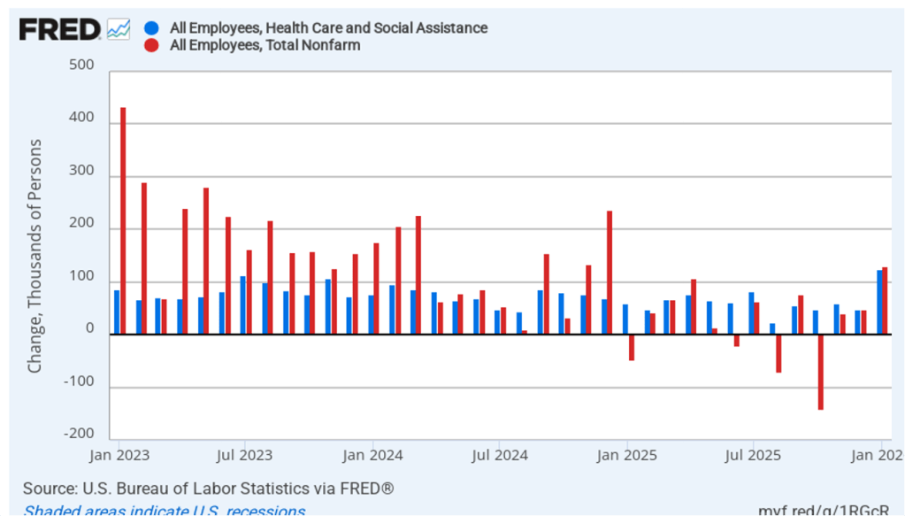
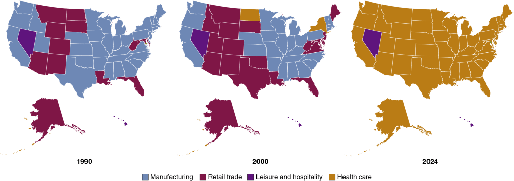
Instead he believes that the key is the continuing strong growth in healthcare jobs, which have traditionally been held disproportionately by females. The availability of these jobs has allowed women to fare better than men in an economy in which hiring rates have been relatively low.

Like most short-run trends, it’s possible that the relatively high unemployment rates experienced by recent college graduates may not continue in the long run.

Solved Problem: Rent Control in Holland

Supports: Microeconomics, MacroeconomicsEconomics, and Essentials of Economics, Chapter 4, Section 4.3

Image generated by ChatGTP-40 of a street in a Dutch city.

An article on bloomberg.com has the headline “How Rent Controls Are Deepening the Dutch Housing Crisis.” The article’s subheadline states that: “A law designed to make homes more affordable ended up aggravating an apartment shortage.” According to the article, the Dutch government passed a law that increased the number of apartments subject to rent control from 80% of all apartments to 96%.

  1. Why might the Dutch government have seen expanding rent control as a way to make apartments more affordable? 
  2. Why might the law have aggravated the shortage of apartments in Holland?

Solving the Problem
Step 1: Review the chapter material. This problem is about the effects of rent control, so you may want to review Chapter 4, Section 4.3, “Government Intervention in the Market: Price Floors and Price Ceilings.”

Step 2: Answer part a. by explaining why the Dutch government may have seen expanding rent control as a way to make apartments more affordable. Figure 4.10 from the textbook shows the effects of rent control. In the example illustrated in the figure, after the government imposes rent control, the 1,900,000 people who are still able to rent an apartment pay $1,500 per month rather than $2,500 per month. For these people, rent control has made apartments more affordable.

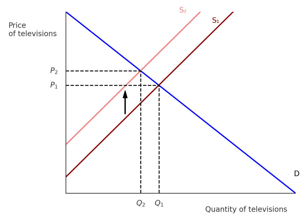
Step 3: Answer part b. by explaining why rent control laws can make an apartment shortage worse. As Figure 4.10 shows, rent control laws impose a price ceiling below the equilibrium market rent. The result is that the quantity of apartments supplied is less than the quantity of apartments demanded, causing a shortage of apartments. In the case of the Dutch law discussed in the article, existing rent controls were expanded to cover more apartments, forcing the rents charged by landlords for these apartments to fall below what had been the equilibrium market rent, thereby adding to the shortage of apartments in Holland.

Extra credit: The article notes that as a result of the law, some owners of apartments that had previously not been subject to rent control had decided to sell their apartments, taking them off the rental market. That result is common when governments impose rent control or expand the scope of an existing rent control law. One important aspect of rent control is that a shortage of apartments gives landlords a greater opportunity to pick and choose the tenants they prefer. The article notes that a provision of the new law requires that rental contracts be open-ended, rather than for only one or two years, as is more common. As a result, landlords have more difficulty evicting tenants who might be noisy or causing other problems. The law thereby gives landlords an incentive to rent to foreign tenants who would be more likely to give up their apartments voluntarily after a year or two. The result is even fewer apartments available for Dutch residents to rent.

A recent article on bloomberg.com notes that the negative consequences of the law expanding rent control has led the Dutch government to propose modifying the law to allow landlords to charge higher rents on at least some apartments. If passed by the Dutch parliment, the changes would go into effect January 1, 2026.

Solved Problem: Do Some Cable Companies Engage in Price Discrimination?

Supports: Microeconomics and Economics, Chapter 15, Section 15.5, and Essentials of Economics, Chapter 10, Section 10.5

Image generated by ChatGTP-4o

A national provider of cable television and internet service has been frequently criticized by customers on social media for using the following business strategy: The company raises its prices every six to nine months. Any subscriber who calls to complain is offered a discount off of the price increase. Analyze how this strategy can be profit mazimizing for the company.

Step 1: Review the chapter material. This problem is about firms using price discrimination, so you may want to review Chapter 15, Sections 15.5 

Step 2: Answer the question by explaining how the cable company is using price discrimination to increase its profit. Price discrimination involves charging different prices to different customers for the same good or service when the price difference isn’t due to differences in cost. Firms who able to price discriminate increase their profits by doing so.

We’ve seen that there are three requirements for a firm to practice price discrimination: 1) The firm must possess market power, 2) some of the firm’s customers much have a greater willingness to pay for the product than do other customers, and 3) the firm must be able to segment the market to keep customers who buy the product at the low price from reselling it. Cable companies can meet all three requirements. Cable firms possess market power—they  aren’t perfect competitors. Some customers have a higher willingness than other customers to pay for cable service. In fact, many people have become cable cutters and prefer to stream content rather than watch programs on cable. Finally, someone who receives a lower-priced cable subscription can’t resell it.

To increase profit by price discrimination, a firm needs to charger a higher price to customers with a lower price elasticity of demand, and a lower price to customers with a higher price elasticity of demand. People who call up to complain about an increase in the price of a cable subscription are likely to be more price sensitive—and, therefore, more likely to switch to a competing cable company or to cut the cable and switch to streaming—than are people who don’t complain about the increase in the price of a subscription. In other words, the complainers have a higher price elasticity of demand than do the non-complainers and receive a lower price. We can conclude that this business strategy is an example of price discrimination and will increase the profit of the cable company that uses it.

Data on the Economics Major

Image generated by ChatGTP-4o.

How does the number of people who majored in economics in college compare with the number of people who pursued other majors? How do the earnings of economics majors compare with the earnings of other majors? Recent data released by the Census Bureau provides some interesting answers to these and other questions about the economics major.

Each year the Census Bureau conducts the American Community Survey (ACS) by mailing a questionnaire to about 3.5 million households. The questionnaire contains 100 questions that ask about, among other things, the race, sex, age, educational attainment, employment, earnings, and health status of each person in the household.  Responses are collected online, by mail, by telephone, or by a personal visit from a census employee.

Although the Census Bureau releases some data about 1 year after the data is collected, it typically takes longer to publish detailed studies of specific topics. The ACS report on Field of Bachelor’s Degree in the United States: 2022 was released this month, although it’s based on data collected during 2022. Anyone interested in the subject will find the whole report to be worthwhile reading, but we can summarize a few of the results.

According to the census, in 2022, there were 81.9 million people in the United States aged 25 and older who had graduated from college with a bachelor’s degree. The report includes economics, along with several other social sciences—psychology, political science, and sociology—in the category of “Engineering and Science Degrees.” The following figure shows the leading majors in this category ranked by the percentage of all holders of a bachelor’s degree. (Sociology is included for comparison with the other three social sciences listed.) Psychology has the largest share of majors at 4.6 percent. Economics accounts for 2.0 percent of majors.

We can conclude that among social science majors, economics is less than half as popular as psychology, slightly less popular than political science, and significantly more popular than sociology.

Economics departments are sometimes located in undergraduate business colleges. The following figure compares economics to other majors listed in the “Business Degrees” category of the report. At nearly 6 percent of all majors, “business management and administration” is the most popular of business majors, followed by general business and accounting. “Other business,” marketing, finance, and economics are all about equally popular with around 2 percent of all majors.

The figure below shows the median annual earnings for people aged 25 years to 64 years—prime-age workers—who majored in each of fields used in the first figure above, as well as for all holders of a bachelor’s degree. People who majored in economics earn significantly more than people who majored in the other social sciences listed and 35 percent more than people in all majors.

 The next figure shows median annual earnings for economics majors compared with majors in other business fields. Perhaps surprisingly—although not to people who know the many benefits from majoring in economics!—economics majors earn more on average than do majors in other business fields.

The following figure shows how many people with bacherlor’s degrees in economics majors fall into each age group. People aged 25 years to 34 years make up 22 percent of all economics majors, the most of any of the age groups. This result indicates that the economics major has gained in popularity (although note that the age groups don’t have equal numbers of people in them).

Finally, we can look at the demographic characteristics of economics majors. The next figure shows the percentage of degree holders in some popular majors who are women. Although women hold 53 percent of all bachelor’s degrees, they hold only 33 percent of bachelor’s degrees in economics. The share for economics is lower than for the other social sciences shown, the same as for finance majors, and more than for computer science and mechanical engineering majors.

The next figure shows bachelor’s degrees in economics by race and Hispanic origin. Non-Hispanic whites and non-Hispanic Asians are overrepresented among economics majors compared with the percentages they make up of all bachelor’s degree holders. Non-Hispanic Blacks and Hispanics are underrepresented among economics majors compared with the percentages they make up of all bachelor’s degree holders. People who are multiracial or of another race hold the same percentage of economics degrees as of degrees in other subjects.