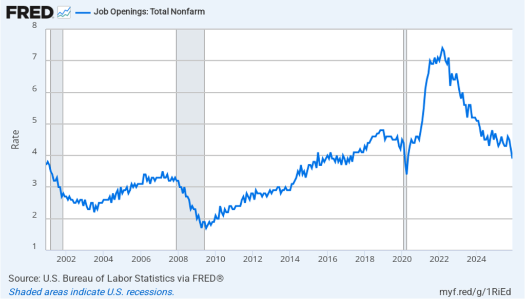
Today (February 5), the Bureau of Labor Statistics (BLS) released its “Job Openings and Labor Turnover” (JOLTS) report for December 2025. The report indicated that labor market conditions may be weakening. The following figure shows that the rate of job openings fell to 3.9 percent in December from 4.2 percent in November. The rate was 4.5 percent in October. The job openings rate is the lowest since April 2020, at the start of the Covid pandemic. We should note the usual caveat that the monthly JOLTS data is subject to potentially large revisions as the BLS receives more complete data.
(The BLS defines a job opening as a full-time or part-time job that a firm is advertising and that will start within 30 days. The rate of job openings is the number of job openings divided by the number of job openings plus the number employed workers, multiplied by 100.)
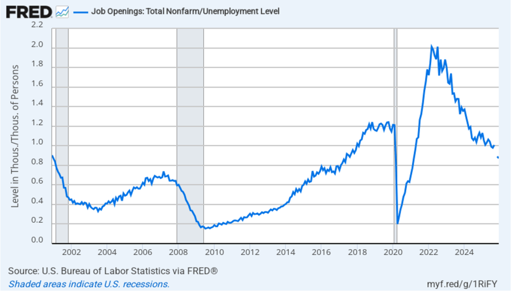
In the following figure, we show a measure of the state of the labor market that economists frequently use: the total number of job openings to the total number of people unemployed. In December there were 0.87 job openings per unemployed person, the lowest value for that measure since March 2021, during the recovery from the pandemic. The value was 1.0 in September. (Note that data for October and November are unavailable because the data weren’t collected during the shutdown of the federal government from October 1 to November 12 last year.) The value for December is well below the 1.21 job openings per employed person in February 2020, just before the pandemic. (Note that, as we discussed in this blog post, the employment-population ratio for prime age workers, which many economists consider a key measure of the state of the labor market, rose in December, putting it above what the ratio was in any month during the period from January 2008 to February 2020.)
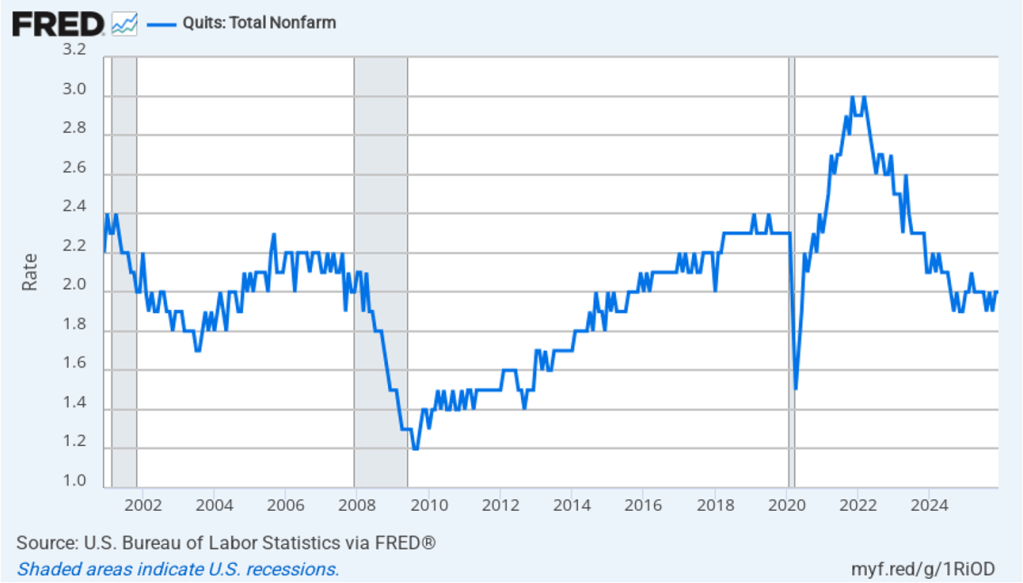
The rate at which workers are willing to quit their jobs is an indication of how they perceive the ease of finding a new job. As the following figure shows, the quit rate declined slowly from a peak of 3 percent in late 2021 and early 2022 to 2.0 percent in August 2024, the same value as in December 2025. That rate is below the rate during 2019 and early 2020. By this measure, workers’ perceptions of the state of the labor market have remained remarkably stable over the last year and a half.
Overall, this JOLTS report is consistent with what some economists have labeled a “slow hire, slow fire” labor market. Fed Chair Jerome Powell’s remarks at his press conference following the last meeting of the Federal Open Market Committee (FOMC) indicates that Fed policymakers share this view, which Powell believes complicates monetary policymaking:
“So there are lots of … little places that suggest that the labor market has softened, but part of … payroll job softening is that both the supply and demand for labor has come down … growth in those two have come down. So that makes it a difficult time to read the labor market. So, imagine they both came down a lot, to the point where there is no job growth. Is that full employment? In a sense it is. If demand and supply are … in balance, you could say that’s full employment. At the same time, is it—do we really feel like … that’s a maximum employment economy? It’s a challenging—it’s very challenging and quite unusual situation.”
The BLS was scheduled to release its monthly “Employment Situation” report (often called the “jobs report”) for January 2026 tomorrow. Because of the temporary lapse in funding that began Saturday, the report will instead be released next Wednesday, February 11. That report will provide additional data on the state of the labor market. (Note that the data in the JOLTS report lag the data in the “Employment Situation” report by one month.)
Image generated by ChatGPT 5 of a 1981 IBM personal computer.
The modern era of information technology began in the 1980s with the spread of personal computers. A key development was the introduction of the IBM personal computer in 1981. The Apple II, designed by Steve Jobs and Steve Wozniak and introduced in 1977, was the first widely used personal computer, but the IBM personal computer had several advantages over the Apple II. For decades, IBM had been the dominant firm in information technology worldwide. The IBM System/360, introduced in 1964, was by far the most successful mainframe computer in the world. Many large U.S. firms depended on IBM to meet their needs for processing payroll, general accounting services, managing inventories, and billing.
Because these firms were often reliant on IBM for installing, maintaining, and servicing their computers, they were reluctant to shift to performing key tasks with personal computers like the Apple II. This reluctance was reinforced by the fact that few managers were familiar with Apple or other early personal computer firms like Commodore or Tandy, which sold the TRS-80 through Radio Shack stores. In addition, many firms lacked the technical staffs to install, maintain, and repair personal computers. Initially, it was easier for firms to rely on IBM to perform these tasks, just as they had long been performing the same tasks for firms’ mainframe computers.
By 1983, the IBM PC had overtaken the Apple II as the best-selling personal computer in the United States. In addition, IBM had decided to rely on other firms to supply its computer chips (Intel) and operating system (Microsoft) rather than develop its own proprietary computer chips and operating system. This so-called open architecture made it possible for other firms, such as Dell and Gateway, to produce personal computers that were similar to IBM’s. The result was to give an incentive for firms to produce software that would run on both the IBM PC and the “clones” produced by other firms, rather than produce software for Apple personal computers. Key software such as the spreadsheet program Lotus 1-2-3 and word processing programs, such as WordPerfect, cemented the dominance of the IBM PC and the IBM clones over Apple, which was largely shut out of the market for business computers.
As personal computers began to be widely used in business, there was a general expectation among economists and policymakers that business productivity would increase. Productivity, measured as output per hour of work, had grown at a fairly rapid average annual rate of 2.8 percent between 1948 and 1972. As we discuss in Macroeconomics, Chapter 10 (Economics, Chapter 20 and Essentials of Economics, Chapter 14) rising productivity is the key to an economy achieving a rising standard of living. Unless output per hour worked increases over time, consumption per person will stagnate. An annual growth rate of 2.8 percent will lead to noticeable increases in the standard of living.
Economists and policymakers were concerned when productivity growth slowed beginning in 1973. From 1973 to 198o, productivity grew at an annual rate of only 1.3 percent—less than half the growth rate from 1948 to 1972. Despite the widespread adoption of personal computers by businesses, during the 1980s, the growth rate of productivity increased only to 1.5 percent. In 1987, Nobel laureate Robert Solow of MIT famously remarked: “You can see the computer age everywhere but in the productivity statistics.” Economists labeled Solow’s observation the “productivity paradox.” With hindsight, it’s now clear that it takes time for businesses to adapt to a new technology, such as personal computers. In addition, the development of the internet, increases in the computing power of personal computers, and the introduction of innovative software were necessary before a significant increase in productivity growth rates occurred in the mid-1990s.
Result when ChatGPT 5 is asked to create an image illustrating ChatGPT
The release of ChatGPT in November 2022 is likely to be seen in the future as at least as important an event in the evolution of information technology as the introduction of the IBM PC in August 1981. Just as with personal computers, many people have been predicting that generative AI programs will have a substantial effect on the labor market and on productivity.
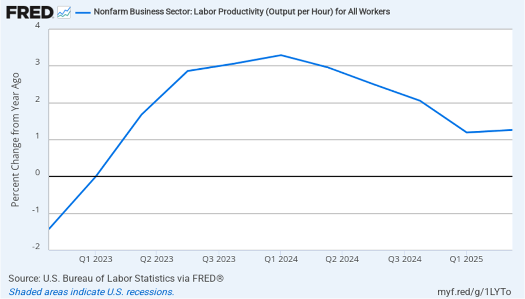
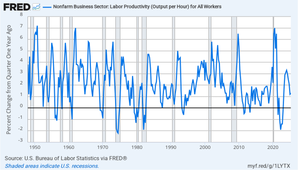
In this recent blog post, we discussed the conflicting evidence as to whether generative AI has been eliminating jobs in some occupations, such as software coding. Has AI had an effect on productivity growth? The following figure shows the rate of productivity growth in each quarter since the fourth quarter of 2022. The figure shows an acceleration in productivity growth beginning in the fourth quarter of 2023. From the fourth quarter of 2023 through the fourth quarter of 2024, productivity grew at an annual rate of 3.1 percent—higher than during the period from 1948 to 1972. Some commentators attributed this surge in productivity to the effects of AI.
However, the increase in productivity growth wasn’t sustained, with the growth rate in the first half of 2025 being only 1.3 percent. That slowdown makes it more likely that the surge in productivity growth was attributable to the recovery from the 2020 Covid recession or was simply an example of the wide fluctuations that can occur in productivity growth. The following figure, showing the entire period since 1948, illustrates how volatile quarterly rates of productivity growth are.
How large an effect will AI ultimately have on the labor market? If many current jobs are replaced by AI is it likely that the unemployment rate will soar? That’s a prediction that has often been made in the media. For instance, Dario Amodei, the CEO of generative AI firm Anthropic, predicted during an interview on CNN that AI will wipe out half of all entry level jobs in the U.S. and cause the unemployment rate to rise to between 10% and 20%.
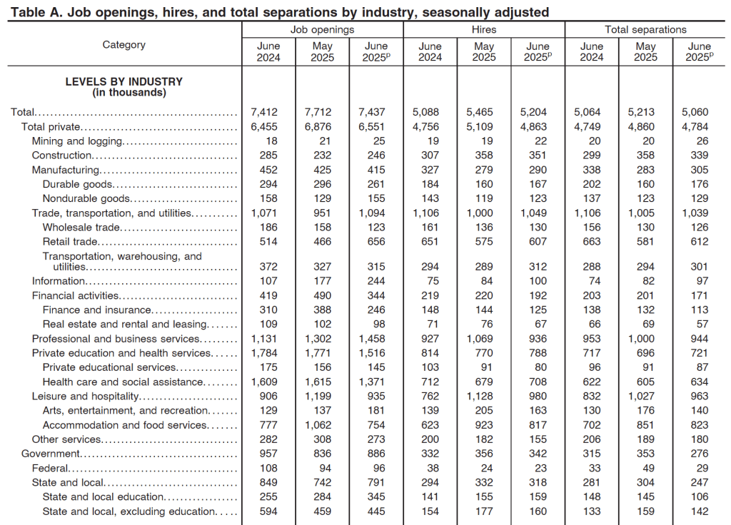
Although Amodei is likely correct that AI will wipe out many existing jobs, it’s unlikely that the result will be a large increase in the unemployment rate. As we discuss in Macroeconomics, Chapter 9 (Economics, Chapter 19 and Essentials of Economics, Chapter 13) the U.S. economy creates and destroys millions of jobs every year. Consider, for instance, the following table from the most recent “Job Openings and Labor Turnover” (JOLTS) report from the Bureau of Labor Statistics (BLS). In June 2025, 5.2 million people were hired and 5.1 million left (were “separated” from) their jobs as a result of quitting, being laid off, or being fired.
Most economists believe that one of the strengths of the U.S. economy is the flexibility of the U.S. labor market. With a few exceptions, “employment at will” holds in every state, which means that a business can lay off or fire a worker without having to provide a cause. Unionization rates are also lower in the United States than in many other countries. U.S. workers have less job security than in many other countries, but—crucially—U.S. firms are more willing to hire workers because they can more easily lay them off or fire them if they need to. (We discuss the greater flexibility of U.S. labor markets in Macroeconomics, Chapter 11 (Economics, Chapter 21).)
The flexibility of the U.S. labor market means that it has shrugged off many waves of technological change. AI will have a substantial effect on the economy and on the mix of jobs available. But will the effect be greater than that of electrification in the late nineteenth century or the effect of the automobile in the early twentieth century or the effect of the internet and personal computing in the 1980s and 1990s? The introduction of automobiles wiped out jobs in the horse-drawn vehicle industry, just as the internet has wiped out jobs in brick-and-mortar retailing. People unemployed by technology find other jobs; sometimes the jobs are better than the ones they had and sometimes the jobs are worse. But economic historians have shown that technological change has never caused a spike in the U.S. unemployment rate. It seems likely—but not certain!—that the same will be true of the effects of the AI revolution.
Which jobs will AI destroy and which new jobs will it create? Except in a rough sense, the truth is that it is very difficult to tell. Attempts to forecast technological change have a dismal history. To take one of many examples, in 1998, Paul Krugman, later to win the Nobel Prize, cast doubt on the importance of the internet: “By 2005 or so, it will become clear that the Internet’s impact on the economy has been no greater than the fax machine’s.” Krugman, Amodei and other prognosticators of the effects of technological change simply lack the knowledge to make an informed prediction because the required knowledge is spread across millions of people.
That knowledge only becomes available over time. The actions of consumers and firms interacting in markets mobilize information that is initially known only partially to any one person. In 1945, Friedrich Hayek made this argument in “The Use of Knowledge in Society,” which is one of the most influential economics articles ever written. One of Hayek’s examples is an unexpected decrease in the supply of tin. How will this development affect the economy? We find out only by observing how people adapt to a rising price of tin: “The marvel is that … without an order being issued, without more than perhaps a handful of people knowing the cause, tens of thousands of people whose identity could not be ascertained by months of investigation are made [by the increase in the price of tin] to use the material or its products more sparingly.” People adjust to changing conditions in ways that we lack sufficient information to reliably forecast. (We discuss Hayek’s view of how the market system mobilizes the knowledge of workers, consumers, and firms in Microeconomics, Chapter 2.)
It’s up to millions of engineers, workers, and managers across the economy, often through trial and error, to discover how AI can best reduce the cost of producing goods and services or improve their quality. Competition among firms drives them to make the best use of AI. In the end, AI may result in more people or fewer people being employed in any particular occupation. At this point, there is no way to know.
“Artificial intelligence is profoundly limiting some young Americans’ employment prospects, new research shows.” That’s the opening sentence of a recent opinion column in the Wall Street Journal. The columnist was reacting to a new academic paper by economists Erik Brynjolfsson, Bharat Chandar, and Ruyu Chen of Stanford University. (See also this Substack post by Chandar that summarizes the results of their paper.) The authors find that:
“[S]ince the widespread adoption of generative AI, early-career workers (ages 22-25) in the most AI-exposed occupations have experienced a 13 percent relative decline in employment … In contrast, employment for workers in less exposed fields and more experienced workers in the same occupations has remained stable or continued to grow. Furthermore, employment declines are concentrated in occupations where AI is more likely to automate, rather than augment, human labor.”
The authors conclude that “our results are consistent with the hypothesis that generative AI has begun to significantly affect entry-level employment.”
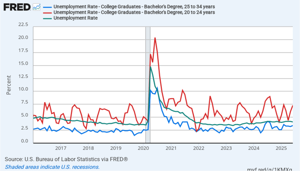
About a month ago, we wrote a blog post looking at whether unemployment among young college graduates has been abnormally high in recent months. The following figure from that post shows that over time, the unemployment rates for the youngest college graduates (the red line) is nearly always above the unemployment rate for the population as a whole (the green line), while the unemployment rate for college graduates 25 to 34 years old (the blue line) is nearly always below the unemployment rate for the population as a whole. In July of this year, the unemployment rate for the population as a whole was 4.2 percent, while the unemployment for college graduates 20 to 24 years old was 8.5 percent, and the unemployment rate for college graduates 25 to 34 years old was 3.8 percent.
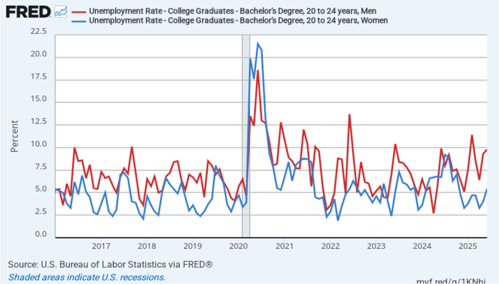
As the following figure (also reproduced from that blog post) shows, the increase in unemployment among young college graduates has been concentrated among males. Does higher male unemployment indicate that AI is eliminating jobs, such as software coding, that are disproportionately male? Data journalist John Burn-Murdoch argues against this conclusion, noting that data shows that “early-career coding employment is now tracking ahead of the [U.S.] economy.”
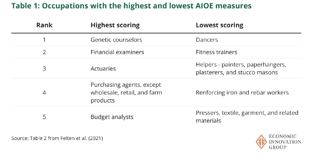
Another recent paper written by Sarah Eckhardt and Nathan Goldschlag of the Economic Innovation Group is also skeptical of the view that firms adopting generative AI programs is reducing employment in certain types of jobs. They use a measure developed by Edward Felton on Princeton University, and Manav Raj and Robert Seamans of New York University of how exposed particular jobs are to AI (AI Occupational Exposure (AIOE)). The following table from Eckhardt and Goldschlag’s paper shows the five most AI exposed jobs and the five least AI exposed jobs.
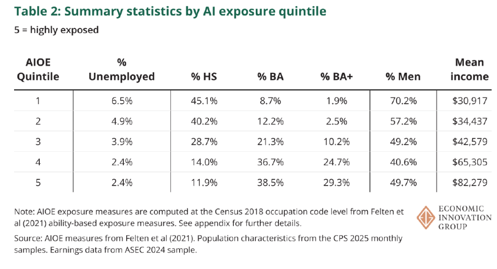
They divide all occupations into quintiles based on the exposure of the occupations to AI. Their key results are given in the following table, which shows that the occupations that are most exposed to the effects of AI—quintiles 4 and 5—have lower unemployment rates and higher wages than do the occupations that are least exposed to AI.
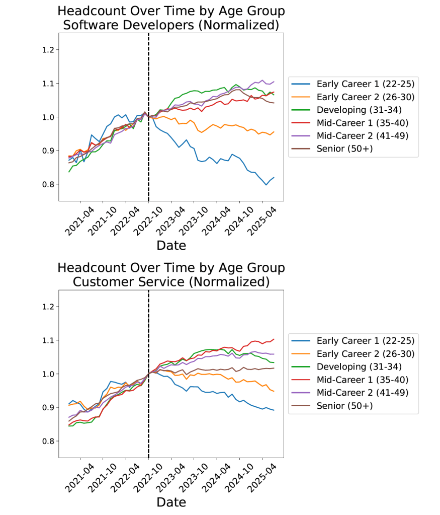
The Brynjolfsson, Chandar, and Chen paper mentioned at the beginning of this post uses a larger data set of workers by occupation from ADP, a private firm that processes payroll data for about 25 percent of U.S. workers. Figure 1 from their paper, reproduced here, shows that employment of workers in two occupations—software developers and customer service—representative of those occupations most exposted to AI declined sharply after generative AI programs became widely available in late 2022.
They don’t find this pattern for all occupations, as shown in the following figure from their paper.
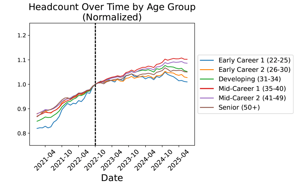
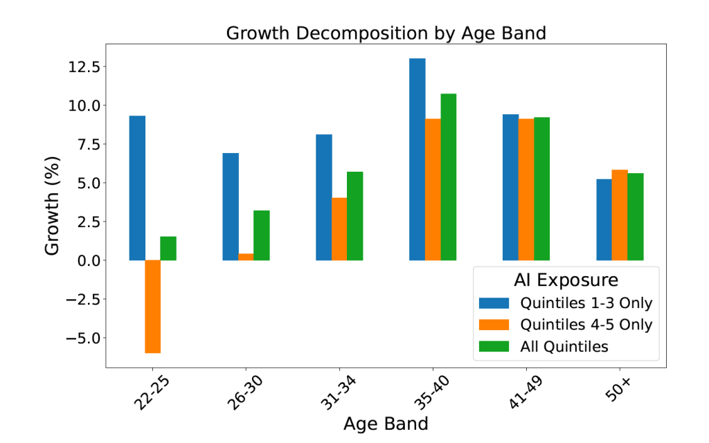
Finally, they show results by occupational quintiles, with workers ages aged 22 to 25 being hard hit in the two occupational quintiles (4 and 5) most exposted to AI. The data show total employment growth from October 2022 to July 2025 by age group and exposure to AI.
Economics blogger Noah Smith has raised an interesting issue about Brynjolfsson, Chandar, and Chen’s results. Why would we expect that the negative effect of AI on employment to be so highly concentrated among younger workers? Why would employment in the most AI exposed occupations be growing rapidly among workers aged 35 and above? Smith wonders “why companies would be rushing to hire new 40-year-old workers in those AI-exposed occupations.” He continues:
“Think about it. Suppose you’re a manager at a software company, and you realize that the coming of AI coding tools means that you don’t need as many software engineers. Yes, you would probably decide to hire fewer 22-year-old engineers. But would you run out and hire a ton of new 40-year-old engineers?“
Both the papers discussed here are worth reading for their insights on how the labor market is evolving in the generative AI era. But taken together, they indicate that it is probably too early to arrive at firm conclusions about the effects of generative AI on the job market for young college graduates or other groups.
Supports: Macroeconomics, Chapter 9,Economics, Chapter 19, and Essentials of Economics, Chapter 13.
Image generated by ChatGPT
A recent article on axios.com notes that from April 2023 to July 2024, the U.S. economy generated an average net increase of 177,000 jobs per month. Despite that job growth, the unemployment rate during that period increased by 0.8 percentage point. The article observes that: “At first glance, the combination of a rising unemployment rate and strong jobs growth simply does not compute.” How is it possible during a given period for both total employment and the unemployment rate to increase?
Solving the Problem Step 1: Review the chapter material. This problem is about calculating the unemployment rate, so you may want to review Chapter 9, Section 9.1, “Measuring the Unemployment Rate, the Labor Force Participation Rate, and the Employment-Population Ratio.”
Step 2: Answer the question by explaining how it’s possible for both the total number of people employed and the unemployment rate to both increase during the same period. The unemployment rate is equal to the number of people unemployed divided by the number of people in the labor force (multiplied by 100). The labor force equals the sum of the number of people employed and the number of people unemployed.
Let’s consider the situation in a particular month. Suppose that the unemployment rate in the previous month was 4 percent. If, during the current month, both the number of people employed and the number of people unemployed increase, the unemployment rate will increase if the increase in the number of people unemployed as a percentage of the increase in the labor force is greater than 4 percent. The unemployment rate will decrease if the increase in the number of people unemployed as a percentage of the increase in the labor force is less than 4 percent.
Consider a simple numerical example. Suppose that in the previous month there were 96 people employed and 4 people unemployed. In that case, the unemployment rate was (4/(96 + 4)) x 100 = 4.0%.
Suppose that during the month the number of people employed increases by 30 and the number of people unemployed increases by 1. In that case, there are now 126 people employed and 5 people unemployed. The unemployment rate will have fallen from 4.0% to (5/(126 + 5)) x 100 = 3.8%.
Now suppose that the number of people employed increased by 30 and the number of people unemployed increases by 3. The unemployment will have risen from 4.0% to (7/(126 + 7)) x 100 = 5.3%.
We can conclude that if both the total number of people employed and the total number of people unemployed increase during a during a period of time, it’s possible for the unemployment rate to also increase.
As we noted in yesterday’s blog post, the latest “Employment Situation” report from the Bureau of Labor Statistics (BLS) included very substantial downward revisions of the preliminary estimates of net employment increases for May and June. The previous estimates of net employment increases in these months were reduced by a combined 258,000 jobs. As a result, the BLS now estimates that employment increases for May and June totaled only 33,000, rather than the initially reported 291,000. According to Ernie Tedeschi, director of economics at the Budget Lab at Yale University, apart from April 2020, these were the largest downward revisions since at least 1979.
The size of the revisions combined with the estimate of an unexpectedly low net increase of only 73,000 jobs in June prompted President Donald Trump to take the unprecedented step of firing BLS Commissioner Erika McEntarfer. It’s worth noting that the BLS employment estimates are prepared by professional statisticians and economists and are presented to the commissioner only after they have been finalized. There is no evidence that political bias affects the employment estimates or other economic data prepared by federal statistical agencies.
Why were the revisions to the intial May and June estimates so large? The BLS states in each jobs report that: “Monthly revisions result from additional reports received from businesses and government agencies since the last published estimates and from the recalculation of seasonal factors.” An article in the Wall Street Journal notes that: “Much of the revision to May and June payroll numbers was due to public schools, which employed 109,100 fewer people in June than BLS believed at the time.” The article also quotes Claire Mersol, an economist at the BLS as stating that: “Typically, the monthly revisions have offsetting movements within industries—one goes up, one goes down. In June, most revisions were negative.” In other words, the size of the revisions may have been due to chance.
Is it possible, though, that there was a more systematic error? As a number of people have commented, the initial response rate to the Current Employment Statistics (CES) survey has been declining over time. Can the declining response rate be the cause of larger errors in the preliminary job estimates?
In an article published earlier this year, economists Sylvain Leduc, Luiz Oliveira, and Caroline Paulson of the Federal Reserve Bank of San Francisco assessed this possibility. Figure 1 from their article illustrates the declining response rate by firms to the CES monthly survey. The figure shows that the response rate, which had been about 64 percent during 2013–2015, fell significantly during Covid, and has yet to return to its earlier levels. In March 2025, the response rate was only 42.6 percent.
The authors find, however, that at least through the end of 2024, the falling response rate doesn’t seem to have resulted in larger than normal revisions of the preliminary employment estimates. The following figure shows their calculation of the average monthly revision for each year beginning with 1990. (It’s important to note that they are showing the absolute values of the changes; that is, negative change are shown as positive changes.) Depite lower response rates, the revisions for the years 2022, 2023, and 2024 were close to the average for the earlier period from 1990 to 2019 when response rates to the CES were higher.
The weak employment numbers correspond to the period after the Trump administration announced large tariff increases on April 2. Larger firms tend to respond to the CES in a timely manner, while responses from smaller firms lag. We might expect that smaller firms would have been more likely to hesitate to expand employment following the tariff announcement. In that sense, it may be unsurprising that we have seen downward revisions of the prelimanary employment estimates for May and June as the BLS received more survey responses. In addition, as noted earlier, an overestimate of employment in local public schools alone accounts for about 40 percent of the downward revisions for those months. Finally, to consider another possibility, downward revisions of employment estimates are more likely when the economy is heading into, or has already entered, a recession. The following figure shows the very large revisisons to the establishment survey employment estimates during the 2007–2010 period.
At this point, we don’t fully know the reasons for the downward employment revisions announced yesterday, although it’s fair to say that they may have been politically the most consequential revisions in the history of the establishment survey.
A number of news stories have highlighted the struggles some recent college graduates have had in finding a job. A report earlier this year by economists Jaison Abel and Richard Deitz at the Federal Reserve Bank of New York noted that: “The labor market for recent college graduates deteriorated noticeably in the first quarter of 2025. The unemployment rate jumped to 5.8 percent—the highest reading since 2021—and the underemployment rate rose sharply to 41.2 percent.” The authors define “underemployment” as “A college graduate working in a job that typically does not require a college degree is considered underemployed.”
The following figure shows data on the unemployment rate for people ages 20 to 24 years (red line) with a bachelor’s degree, the unemployment rate for people ages 25 to 34 years (blue line) with a bachelor’s degree, and the unemployment rate for the whole population (green line) whatever their age and level of education. (Note that the values for college graduates are for those people who have a bachelor’s degree but no advanced degree, such as a Ph.D. or an M.D.)
The figure shows that unemployment rates are more volatile for both categories of college graduates than the unemployment rate for the population as a whole. The same is true for the unemployment rates for nearly any sub-category of the unemployed lagely because the number of people included the sub-categories in the Bureau of Labor Statistics (BLS) household survey is much smaller than for the population as a whole. The figure shows that, over time, the unemployment rates for the youngest college graduates is nearly always above the unemployment rate for the population as a whole, while the unemployment rate for college graduates 25 to 34 years old is nearly always below the unemployment rate for the population as a whole. In June of this year, the unemployment rate for the population as a whole was 4.1 percent, while the unemployment for the youngest college graduates was 7.3 percent.
Why is the unemployment rate for the youngest college graduates so high? An article in the Wall Street Journal offers one explanation: “The culprit, economists say, is a general slowdown in hiring. That hasn’t really hurt people who already have jobs, because layoffs, too, have remained low, but it has made it much harder for people who don’t have work to find employment.” The following figure shows that the hiring rate—defined as the number of hires during a month divided by total employment in that month—has been falling. The hiring rate in June was 3.4 per cent, which—apart from two months at the beginning of the Covid pandemic—is the lowest rate since February 2014.
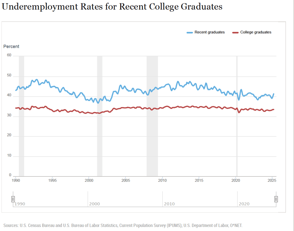
Abel and Deitz, of the New York Fed, have calculated the underemployment for new college graduates and for all college graduates. These data are shown in the following figure from the New York Fed site. The definitions used are somewhat different from the ones in the earlier figures. The definition of college graduates includes people who have advanced degrees and the definition of young college graduates includes people aged 22 years to 27 years. The data are three-month moving averages.
The data show that the underemployment rate for both recent graduates and all graduates are relatively high for the whole period shown. Typically, more than 30 percent of all college graduates and more than 40 percent of recent college graduates work in jobs in which more than 50 percent of employees don’t have college degrees. The latest underemployment rate for recent graduates is the highest since March 2022. It’s lower, though, than the rate for most of the period between the Great Recession of 2007–2009 and the Covid recession of 2020.
In a recent article, John Burn-Murdoch, a data journalist for the Financial Times, has made the point that the high unemployment rates of recent college graduates are concentrated among males. As the following figure shows, in recent months, unemployment rates among male college graduates 20 to 24 years old have been significantly higher than the unemployment rates among female college graduates. In June 2025, the unemployment rate for male recent college graduates was 9.8 percent, well above the 5.4 percent unemployment for female recent college graduates.
What explains the rise in male unemployment relative to female unemployment? Burn-Murdoch notes that, contrary to some media reports, the answer doesn’t seem to be that AI has resulted in a contraction in entry-level software coding jobs that have traditionally been held disproportionately by males. He presents data showing that “early-career coding employment is now tracking ahead of the [U.S.] economy.”
Instead he believes that the key is the continuing strong growth in healthcare jobs, which have traditionally been held disproportionately by females. The availability of these jobs has allowed women to fare better than men in an economy in which hiring rates have been relatively low.
Like most short-run trends, it’s possible that the relatively high unemployment rates experienced by recent college graduates may not continue in the long run.
How does the number of people who majored in economics in college compare with the number of people who pursued other majors? How do the earnings of economics majors compare with the earnings of other majors? Recent data released by the Census Bureau provides some interesting answers to these and other questions about the economics major.
Each year the Census Bureau conducts the American Community Survey (ACS) by mailing a questionnaire to about 3.5 million households. The questionnaire contains 100 questions that ask about, among other things, the race, sex, age, educational attainment, employment, earnings, and health status of each person in the household. Responses are collected online, by mail, by telephone, or by a personal visit from a census employee.
Although the Census Bureau releases some data about 1 year after the data is collected, it typically takes longer to publish detailed studies of specific topics. The ACS report on Field of Bachelor’s Degree in the United States: 2022 was released this month, although it’s based on data collected during 2022. Anyone interested in the subject will find the whole report to be worthwhile reading, but we can summarize a few of the results.
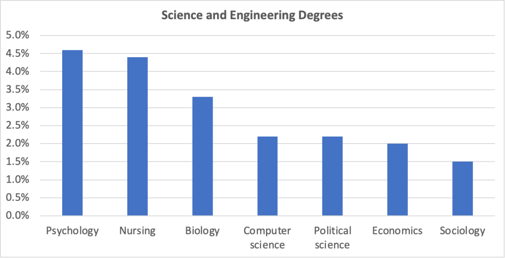
According to the census, in 2022, there were 81.9 million people in the United States aged 25 and older who had graduated from college with a bachelor’s degree. The report includes economics, along with several other social sciences—psychology, political science, and sociology—in the category of “Engineering and Science Degrees.” The following figure shows the leading majors in this category ranked by the percentage of all holders of a bachelor’s degree. (Sociology is included for comparison with the other three social sciences listed.) Psychology has the largest share of majors at 4.6 percent. Economics accounts for 2.0 percent of majors.
We can conclude that among social science majors, economics is less than half as popular as psychology, slightly less popular than political science, and significantly more popular than sociology.
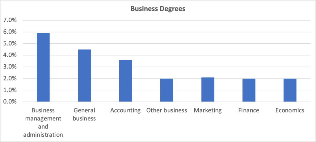
Economics departments are sometimes located in undergraduate business colleges. The following figure compares economics to other majors listed in the “Business Degrees” category of the report. At nearly 6 percent of all majors, “business management and administration” is the most popular of business majors, followed by general business and accounting. “Other business,” marketing, finance, and economics are all about equally popular with around 2 percent of all majors.
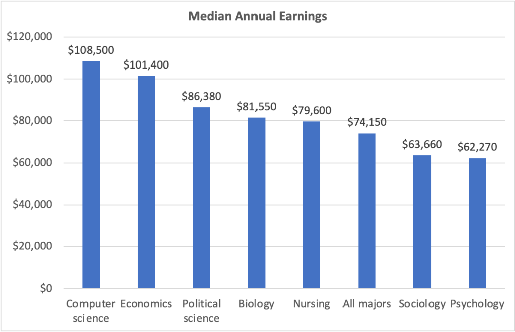
The figure below shows the median annual earnings for people aged 25 years to 64 years—prime-age workers—who majored in each of fields used in the first figure above, as well as for all holders of a bachelor’s degree. People who majored in economics earn significantly more than people who majored in the other social sciences listed and 35 percent more than people in all majors.
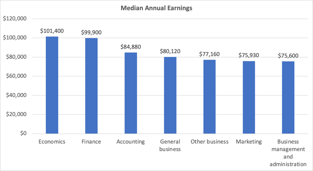
The next figure shows median annual earnings for economics majors compared with majors in other business fields. Perhaps surprisingly—although not to people who know the many benefits from majoring in economics!—economics majors earn more on average than do majors in other business fields.
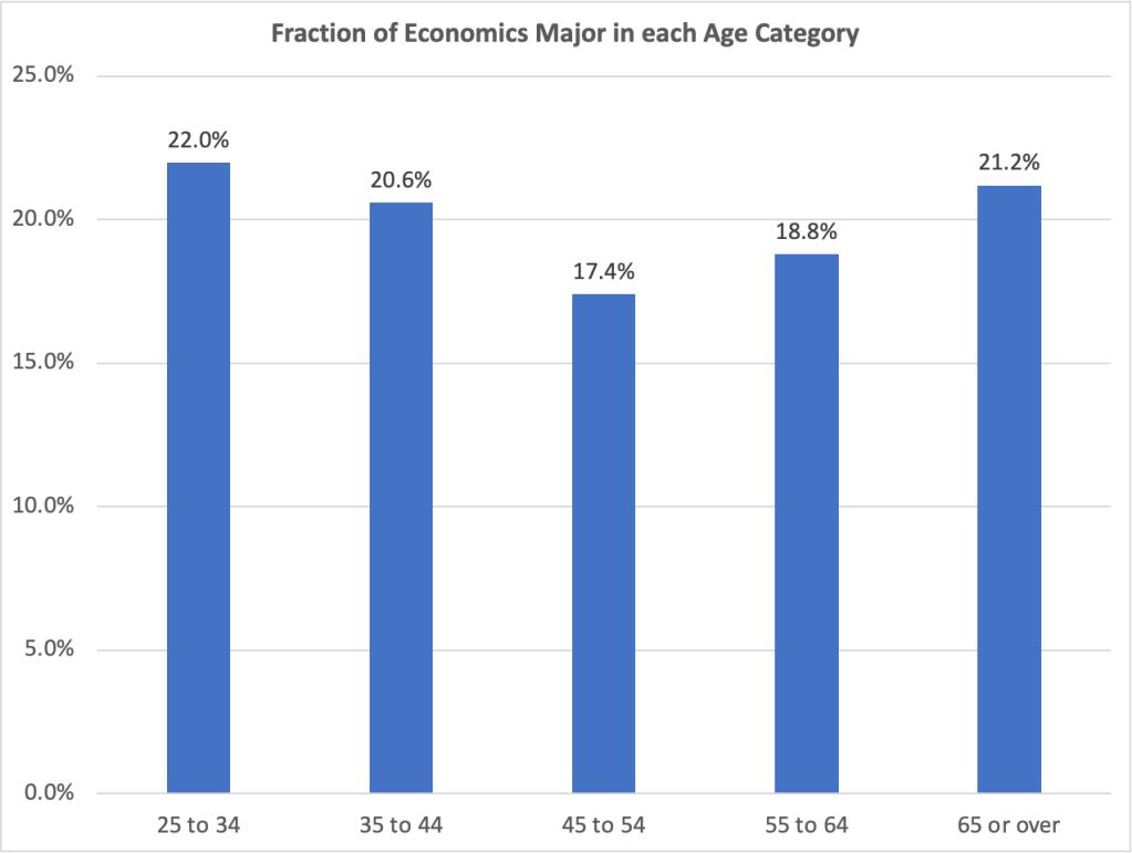
The following figure shows how many people with bacherlor’s degrees in economics majors fall into each age group. People aged 25 years to 34 years make up 22 percent of all economics majors, the most of any of the age groups. This result indicates that the economics major has gained in popularity (although note that the age groups don’t have equal numbers of people in them).
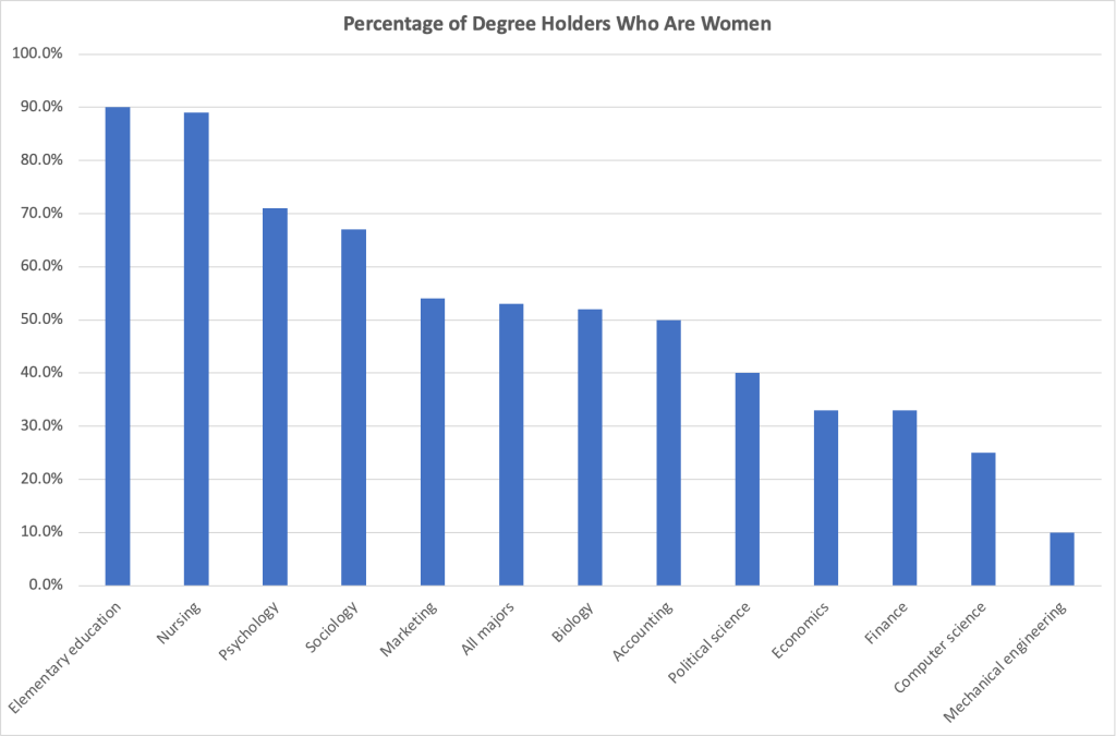
Finally, we can look at the demographic characteristics of economics majors. The next figure shows the percentage of degree holders in some popular majors who are women. Although women hold 53 percent of all bachelor’s degrees, they hold only 33 percent of bachelor’s degrees in economics. The share for economics is lower than for the other social sciences shown, the same as for finance majors, and more than for computer science and mechanical engineering majors.
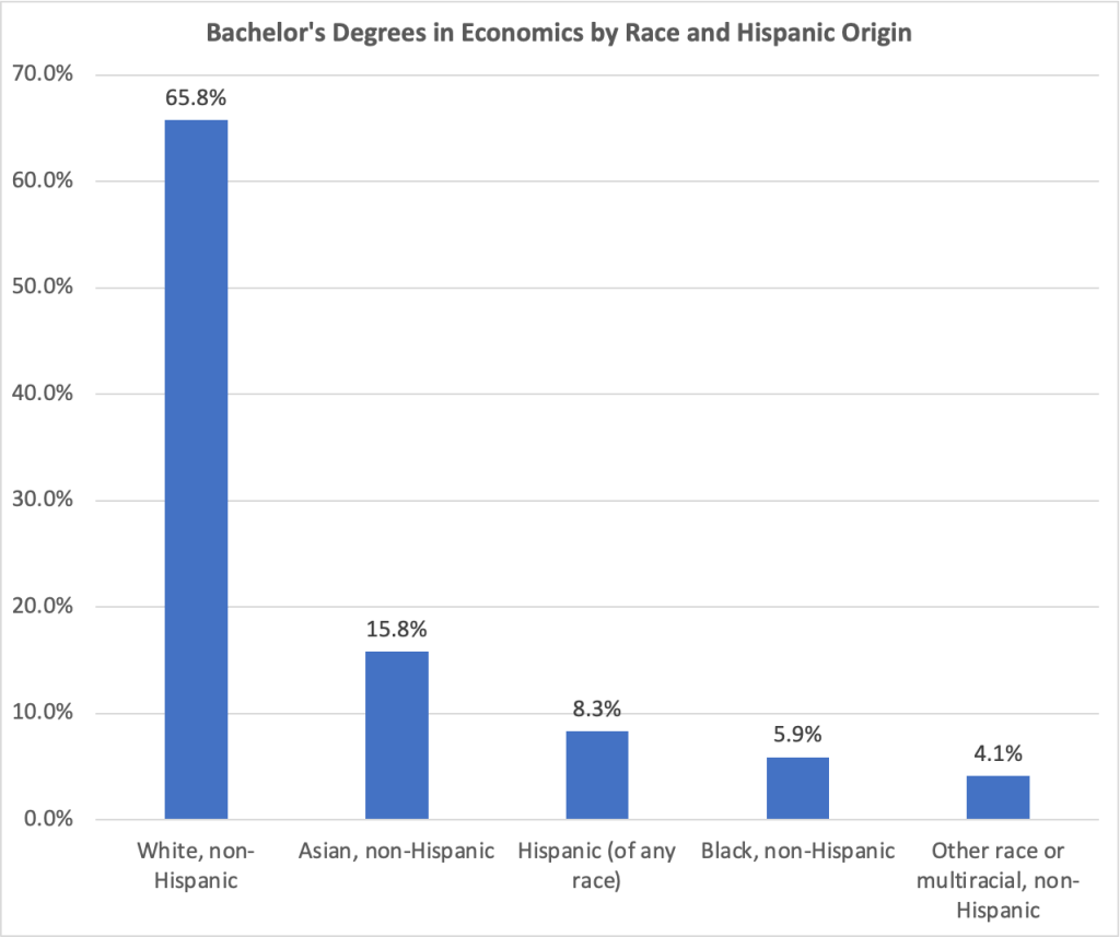
The next figure shows bachelor’s degrees in economics by race and Hispanic origin. Non-Hispanic whites and non-Hispanic Asians are overrepresented among economics majors compared with the percentages they make up of all bachelor’s degree holders. Non-Hispanic Blacks and Hispanics are underrepresented among economics majors compared with the percentages they make up of all bachelor’s degree holders. People who are multiracial or of another race hold the same percentage of economics degrees as of degrees in other subjects.
Photo of Caitlin Clark when she played for the University of Iowa from Reuters via the Wall Street Journal.
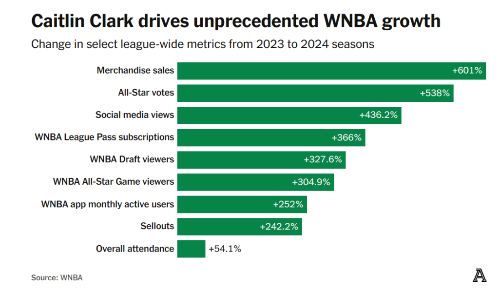
Caitlin Clark’s ability to hit three-point shots made her a star at the University of Iowa. Since she joined the Indiana Fever of the Women’s National Basketball Association (WNBA) in 2024, she’s been, arguably, the league’s biggest star. An article on theathletic.com discussing Clark’s effect on the league includes the following chart:
Clark’s popularity has resulted in substantially increased revenue for her team and for the WNBA. Should that fact affect the salary she receives from the Indiana Fever? The article states that: “Clark will almost assuredly never receive in salary what she is worth to the WNBA. In that regard, she’s a lot like [former men’s basketball star Michael] Jordan, and other all-time greats across sports.” Why won’t Clark be paid a salary equal to her worth to the WNBA?
In Microeconomics, Chapter 16, we show that in a competitive labor market, workers receive the value of their maginal products. The value of a basketball player’s marginal product is the additional revenue the player’s team earns from employing the player. We note that the marginal product of an athlete is the additional number of games the athlete’s team wins by employing the player. The value of a player’s marginal product is the additional revenue the team earns from those additional wins. Teams that win more games attract more fans to watch the teams play—both in person and on television or online. Teams earn revenue from selling tickets, as well as concessions and souvenirs sold in the area. Teams are paid for the rights to broadcast or stream their games. And, as the chart above shows, a player as popular as Clark will increase the game jerseys and other merchandise a team can sell.
We note in Chapter 16 that, once their inital contracts with their teams expire, the best professional athletes tend to sign contracts with teams in larger cities. Although an athlete’s marginal product may be no larger in a big city than in a smaller city, the revenue a team earns from the additional games the team wins from employing a star athlete depends in part on the population of the city the team plays in. Clark’s 2025 salary is only $78,066, far below the value of her marginal product, which is likely at least several million dollars. Her current contract with the Fever lasts through the 2027 season. But even after the contract expires, by league rules, she can’t be paid more than $294,244 by whichever team signs her. (It’s possible that amount may have increased by the time her current contract expires.)
The ceiling on WBNA salaries is far below the average salary in most U.S. men’s professional leagues. For instance, the average salary in the men’s National Basketball Association (NBA) during the 2024–2025 year was nearly $12 million. A low salary cap is common in leagues that are relatively new or that aren’t popular enough to receive large payments for the rights to broadcast or stream their games. For example, men’s Major League Soccer (MLS) has a salary limit of about $6 million per team. The WNBA was founded in 1996 (the NBA was founded in 1946) and, although the broadcast and online viewership for its games has increased, its viewership remains well below the NBA’s viewership.
Clark has been earning millions of dollars from endorisng Nike, Gatoade, and other products. But unless the factors just discussed change, it seems unlikely that she will receive a salary equal to the value of her marginal product to the Fever or any WNBA team she might play for in the future. The excerpt from theathletic.com article that we quoted above, though, compares her salary not to the value of her marginal product to the Fever but to the WNBA as a whole. Are there any circumstances under which we might expect a major sports star to be paid a salary equal to the additional revenue he or she is generating for a league as a whole?
The quotation from the article notes that no “all-time great” players, inclduing Michael Jordan of the NBA, have received salaries equal to the value of their marginal product to the leagues they played in. This outcome shouldn’t be surprising. Returns that entrepreneurs or workers earn in a market system are typically well below the total value they provide to society. For example, in a classic academic paper Nobel laureate William Nordhaus of Yale University estimated that entrepreneurs keep just 2.2 percent of the economic surplus they create by founding new firms. (We discuss the concept of economic surplus in Microeconomics, Chapter 4.) Leaving aside the monetary value of Clark to her team and her league, she has provided substantial consumer surplus to viewers of her games that is not captured by arena ticket prices or cable or streaming subscriptions. As we discuss in Chapter 4, the same is true of most goods and services in competitive markets.
Caitlin Clark, like Amazon founder Jeff Bezos, has only received a small fraction of the economic surplus she has created. (Photo from the Wall Street Journal)
So, although Caitlin Clark is a millionaire as a result of the money she has been paid to endorse products, the actual additional value she has created for her team, her league, and the economy is far greater than the income she earns.
“Clark will almost assuredly never receive in salary what she is worth to the WNBA. In that regard, she’s a lot like [Michael] Jordan, and other all-time greats across sports.”
As we noted in a recent post on the latest jobs report, the Bureau of Labor Statistics (BLS) has updated the population estimates in its household employment survey to reflect the revised population estimates from the Census Bureau. The census now estimates that the civilian noninstitutional population was about 2.9 million larger in December 2024 than it had previously estimated. The original undercount was significantly driven by an underestimate of the increase in the immigrant population.
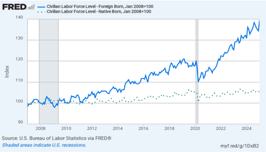
The following figure shows the more rapid growth of foreign-born workers in recent years in comparison with the growth in native-born workers. In the figure, we set the number of native-born workers and the number of foreign-born workers both equal to 100 in January 2007. Between January 2007 and January 2025, the number of foreign-born workers increased by 40 percent, while the number of native-born workers increased by only 6 percent.
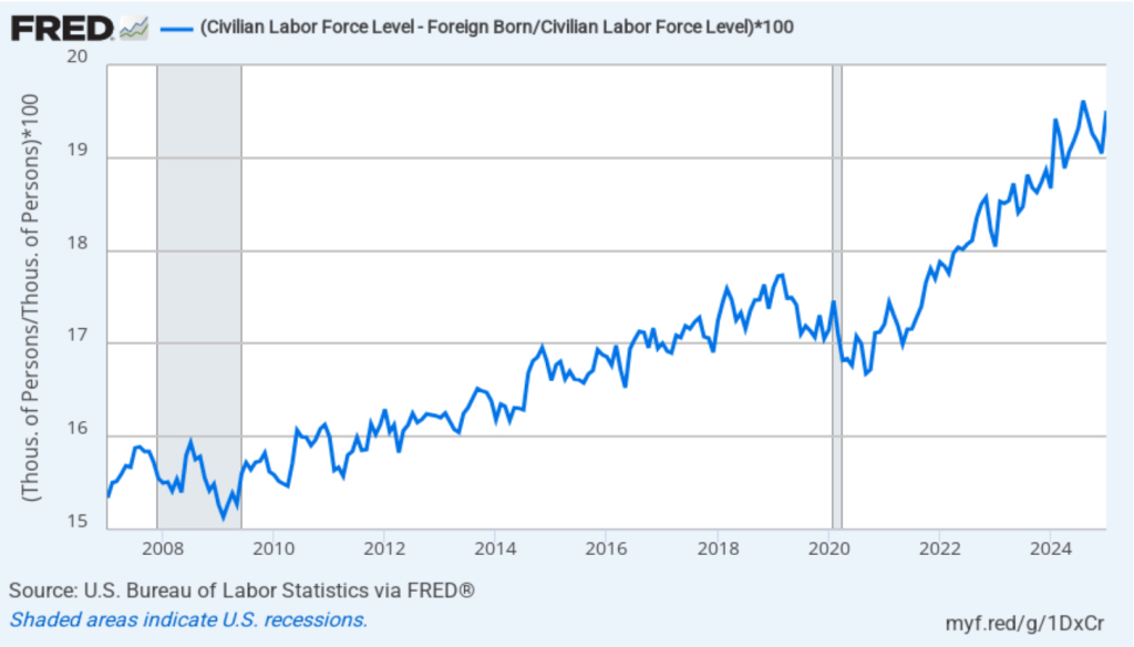
As the following figure shows, although foreign-born workers are an increasingly larger percentage of the total labor force, native-born workers are still a large majority of the labor force. Foreign-born workers were 15.3 percent of the labor force in January 2007 and 19.5 percent of the labor force in January 2025. Foreign-born workers accounted for about 56 percent of the increase in the total labor force over the period from January 2007 to January 2025.
H/T to Jason Furman for pointing us to the BLS data.
At the close of stock trading on Friday, January 24 at 4 pm EST, Nvidia’s stock had a price of $142.62 per share. When trading reopened at 9:30 am on Monday, January 27, Nvidia’s stock price plunged to $127.51. The total value of all Nvidia’s stock (the firm’s market capitalization or market cap) dropped by $589 billion—the largest one day drop in market cap in history. The following figure from the Wall Street Journal shows movements in Nvidia’s stock price over the past six months.
What happened to cause should a dramatic decline in Nvidia’s stock price? As we discuss in Macroeconomics, Chapter 6 (Economics, Chapter 8, and Money, Banking, and the Financial System, Chapter 6), Nividia’s price of $142.62 at the close of trading on January 24—like the price of any publicly traded stock—reflected all the information available to investors about the company. For the company’s stock to have declined so sharply at the beginning of the next trading day, important new information must have become available—which is exactly what happened.
As we discussed in this blog post from last October, Nvidia has been very successful in producing state-of-the-art computer chips that power the most advanced generative artificial intelligence (AI) software. Even after Monday’s plunge in the value of its stock, Nvidia still had a market cap of nearly $3.5 trillion at the end of the day. It wasn’t news that DeepSeek, a Chinese AI company had produced AI software called R1 that was similar to ChatGTP and other AI software produced by U.S. companies. The news was that R1—the latest version of the software is called V3—appeared to be comparable in many ways to the AI software produced by U.S. firms, but had been produced by DeepSeek despite not using the state-of-the-art Nvidia chips used in those AI programs.
The Biden administration had barred export to China of the newest Navidia chips to keep Chinese firms from surging ahead of U.S. firms in developing AI. DeepSeek claimed to have developed its software using less advanced chips and have trained its software at a much lower cost than U.S. firms have been incurring to train their software. (“Training” refers to the process by which engineers teach software to be able to accurately solve problems and answer questions.) Because DeepSeek’s costs are lower, the company charges less than U.S. AI firms do to use its computer infrastructure to handle business tasks like responding to consumer inquiries.
If the claims regarding DeepSeek’s software are accurate, then AI firms may no longer require the latest Nvidia chips and may be forced to reduce the prices they can charge firms for licensing their software. The demand for electricity generation may also decline if it turns out that the demand for AI data centers, which use very large amounts of power, will be lower than expected.
But on Monday it wasn’t yet clear whether the claims being made about DeepSeek’s software were accurate. Some industry observers speculated that, despite the U.S. prohibition on exporting the latest Nvidia chips to China, DeepSeek had managed to obtain them but was reluctant to admit that it had. There were also questions about whether DeepSeek had actually spent as little as it claimed in training its software.
What happens to the price of Nvidia’s stock during the rest of the week will indicate how investors are evaluating the claims DeepSeek made about its AI software.