Image created by ChatGPT of the Department of Commerce building in Washington, DC
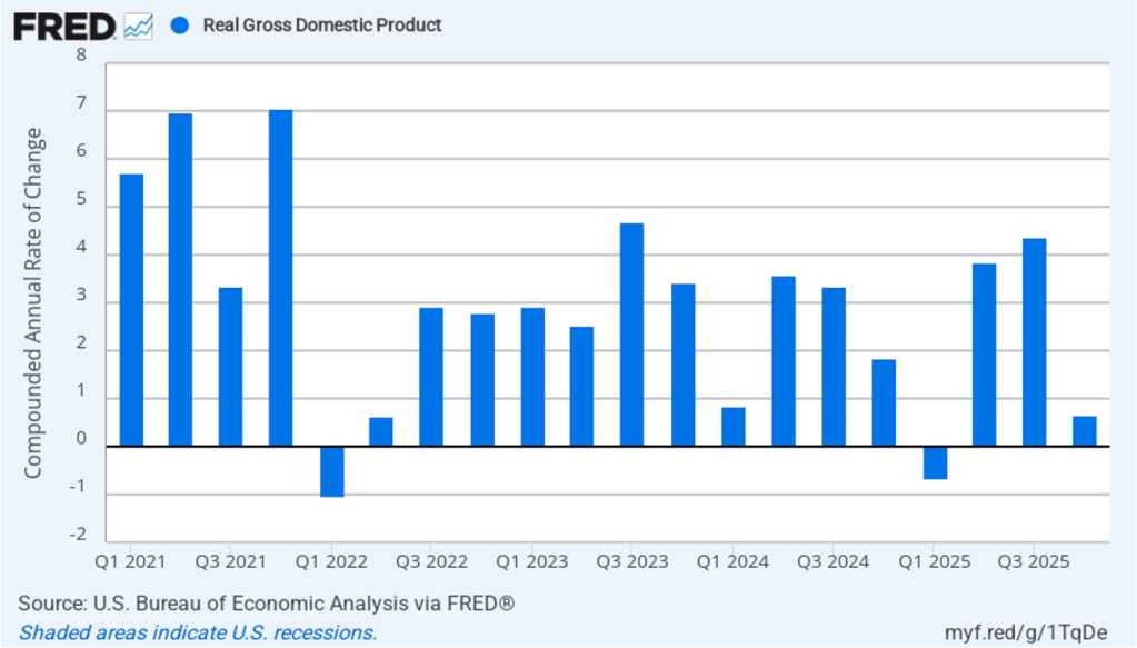
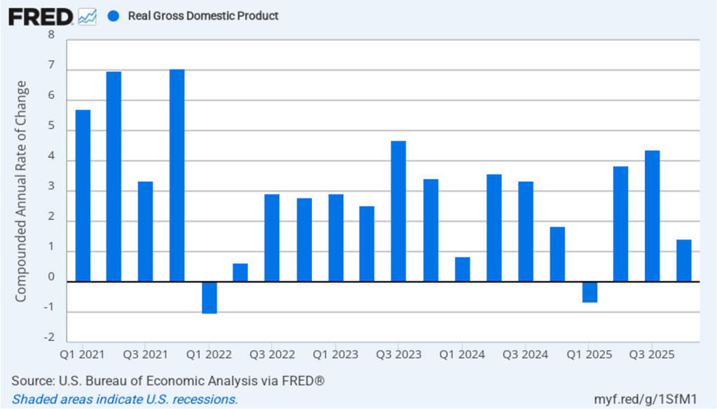
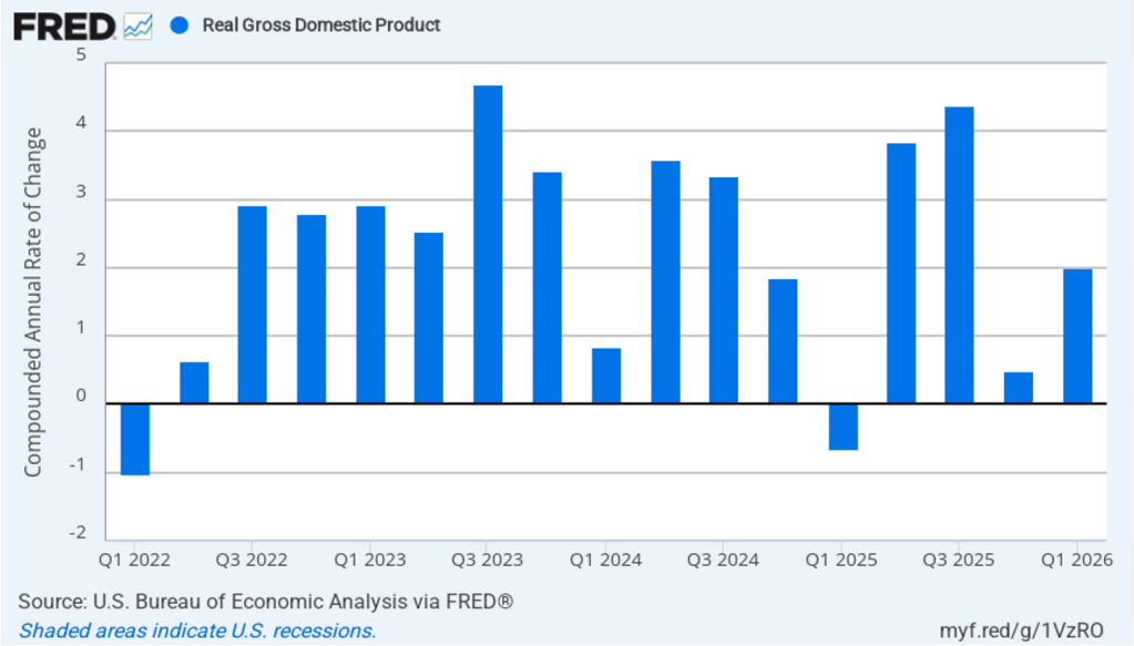
The Bureau of Economic Analysis (BEA) released two reports this morning: “GDP (Advance Estimate), 1st Quarter 2026” and “Personal Income and Outlays, March 2026.” The BEA estimates that real GDP grew at annual rate of 2.0 percent in the first quarter of 2026. That rate was up sharply from 0.5 percent in the fourth quarter of 2025, but below the 2.2 percent rate economists surveyed by the Wall Street Journal had forecast. The following figure shows the BEA’s estimated rates of GDP growth in each quarter beginning with the first quarter of 2022.
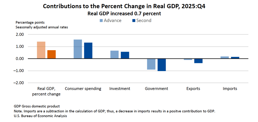
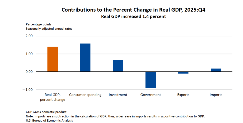
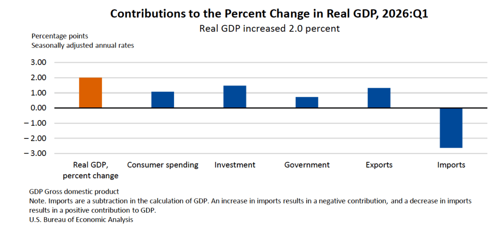
As the following figure—taken from the BEA report—shows, investment spending made the largest contribution to the growth of real GDP in the first quarter, with consumption spending growing at a slower rate than during the previous three quarters. Spending on imports grew significantly more than did spending on exports, resulting in net exports reducing real GDP growth by 1.3 percentage points.
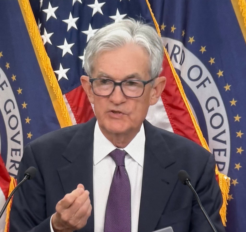
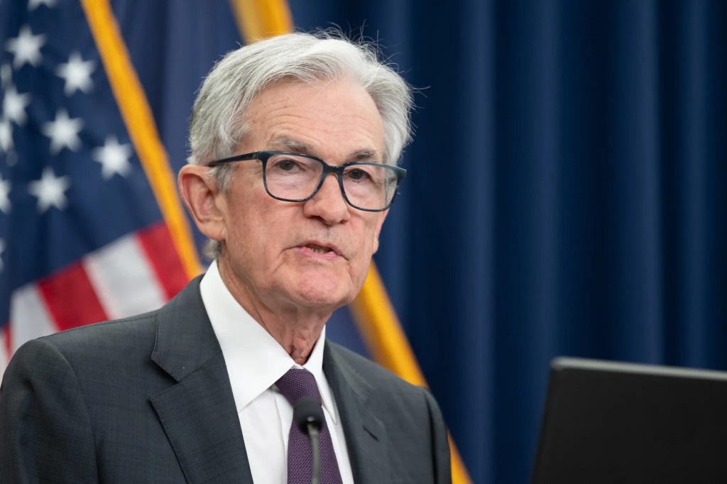
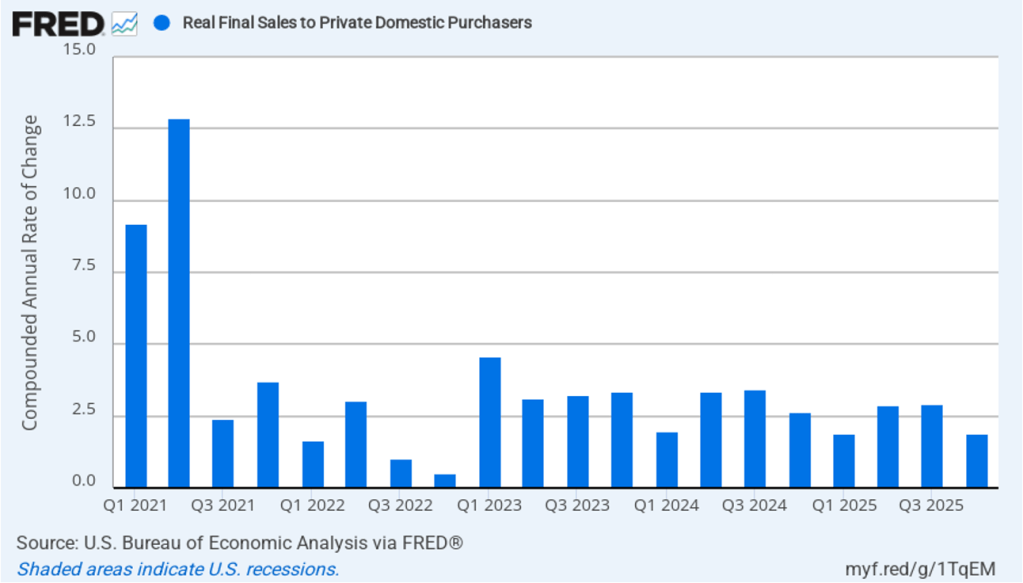
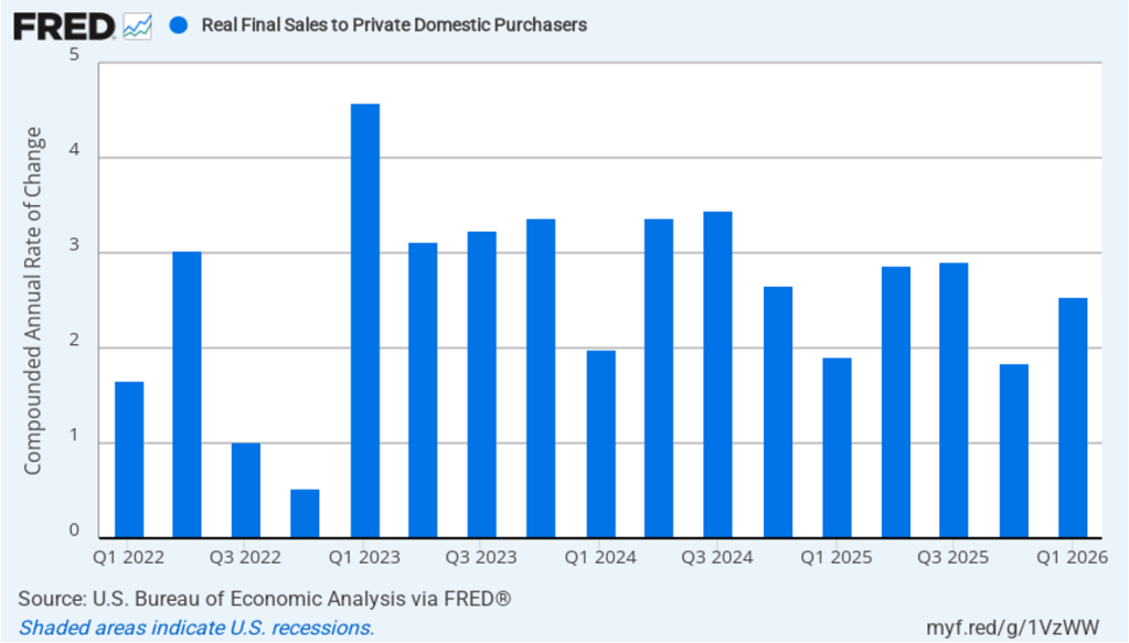
As we’ve discussed in previous blog posts, to better gauge the state of the economy, policymakers—including Fed Chair Jerome Powell—often prefer to strip out the effects of imports, inventory investment, and government expenditures—which can be volatile—by looking at real final sales to private domestic purchasers, which includes only spending by U.S. households and firms on domestic production. As the following figure shows, real final sales to domestic purchasers increased by 2.5 percent at an annual rate in the first quarter, which was well above the 2.0 percent increase in real GDP and also above the U.S. economy’s expected long-run annual real growth rate of 1.8 percent. Note also that real final sales to private domestic purchasers grew by 2.9 percent in the third quarter of 2025, during which real GDP grew by 4.4 percent, and by 1.9 percent in the first quarter of 2025, when real GDP declined by 0.6 percent. So this measure of output is more stable and likely is a better indicator of the underlying growth rate in the economy than is growth in real GDP.
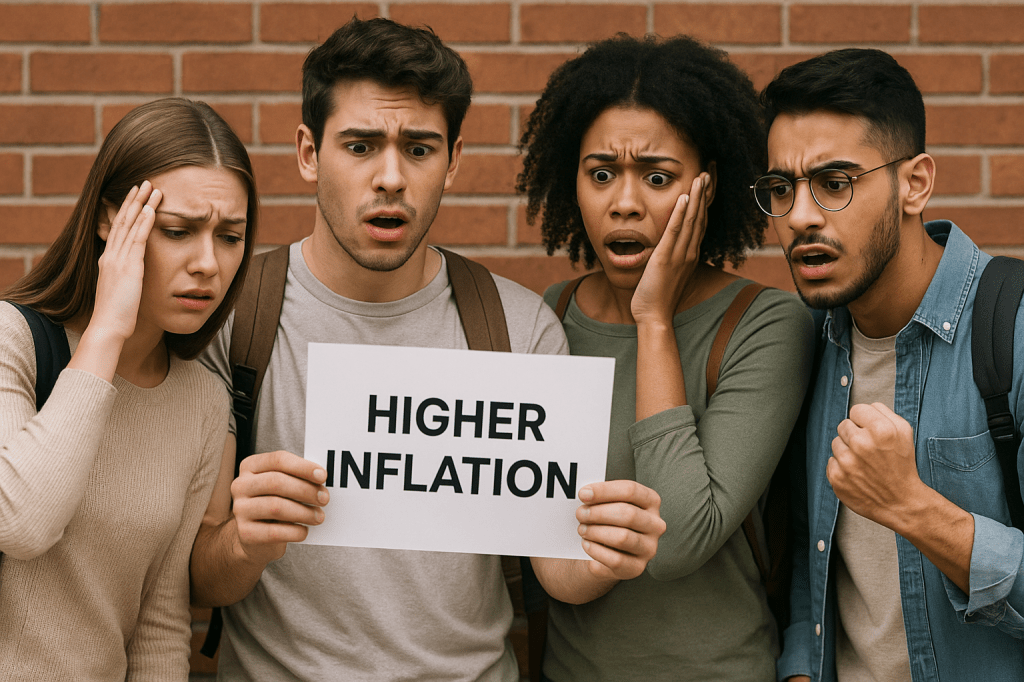
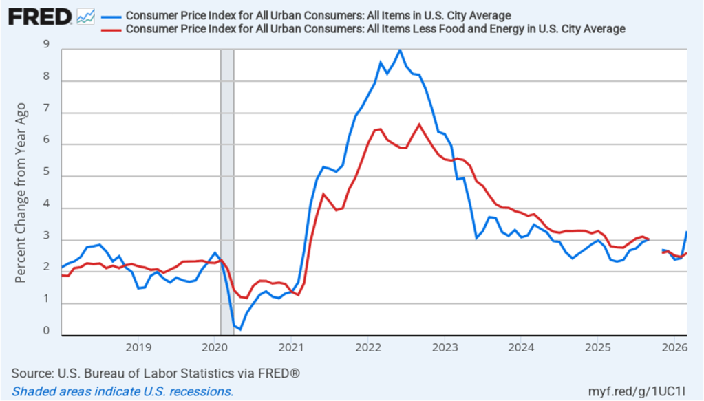
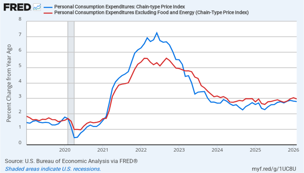
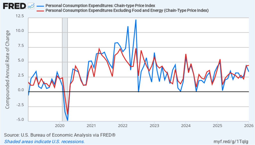
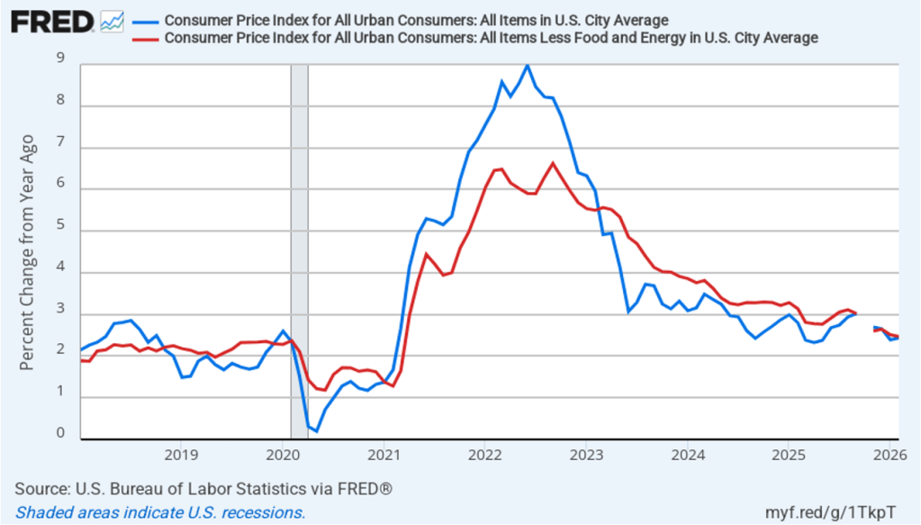
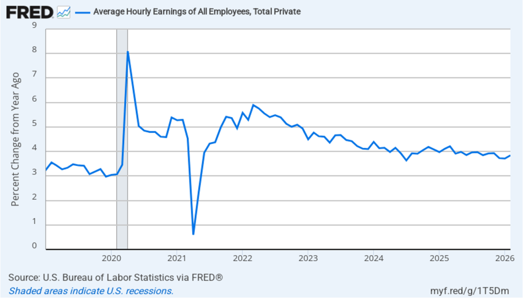
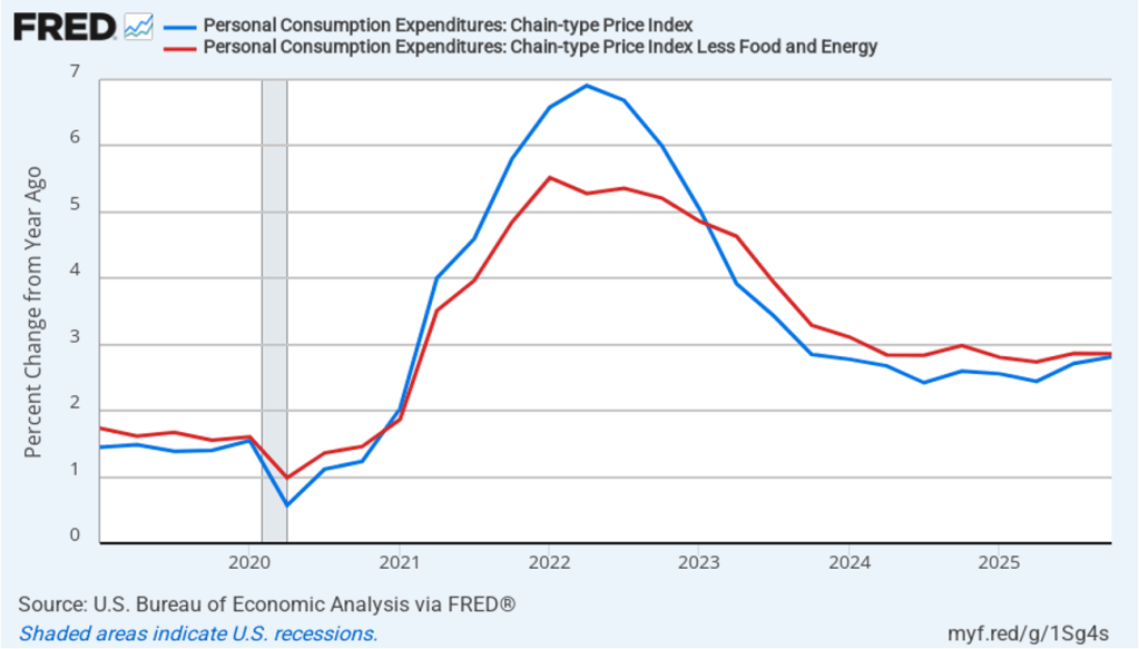
The BEA’s “Personal Income and Outlays” report this morning included monthly data on the personal consumption expenditures (PCE) price index. The Fed relies on annual changes in the PCE price index to evaluate whether it’s meeting its 2 percent annual inflation target. The following figure shows headline PCE inflation (the blue line) and core PCE inflation (the red line)—which excludes energy and food prices—for the period since January 2019, with inflation measured as the percentage change in the PCE from the same month in the previous year. In March, headline PCE inflation was 3.4 percent, up from 2.7 percent in February. Core PCE inflation in March was 3.2 percent, up from 3.0 percent in February. Both headline PCE inflation and core PCE inflation remained well above the Fed’s 2 percent annual inflation target.
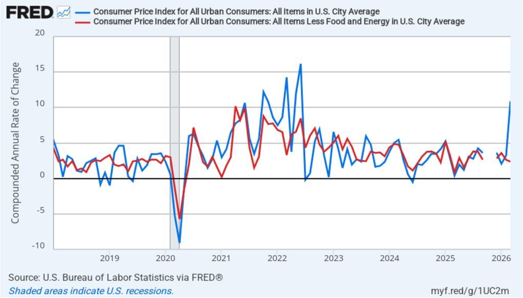
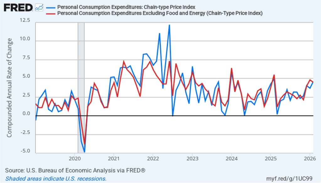
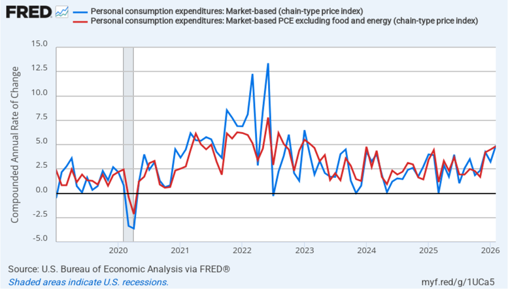
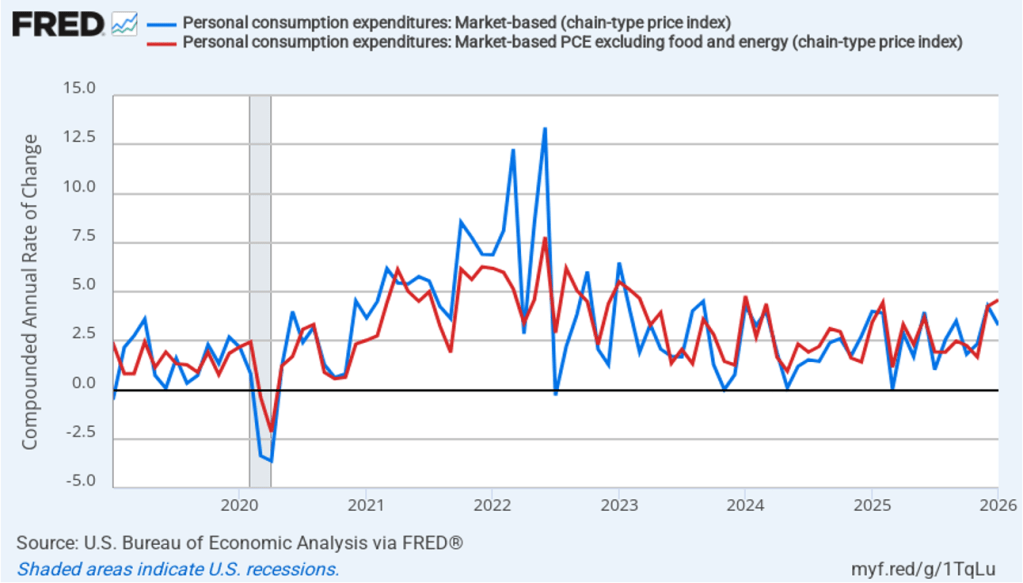
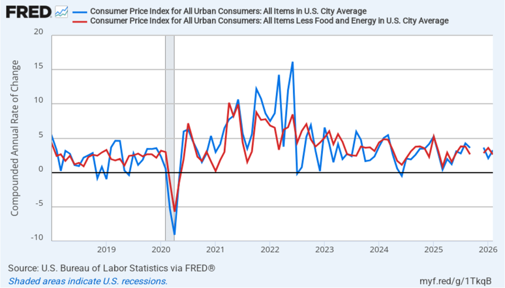
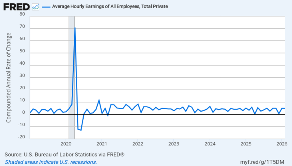
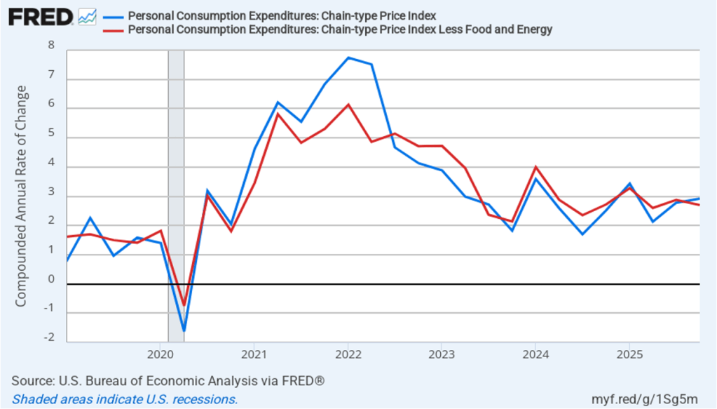
The following figure shows monthly PCE inflation and monthly core PCE inflation calculated by compounding the current month’s rate over an entire year. (Often referred to as 1-month inflation.) Measured this way, headline PCE inflation soared to 9.2 percent in March, up from to 4.9 percent in February. Core PCE inflation fell to 3.6 percent in March from 5.2 percent in February. Even leaving aside the effect of rising gasoline prices on headline PCE, these data show that in March both core and headline PCE inflation were far above the Fed’s target.
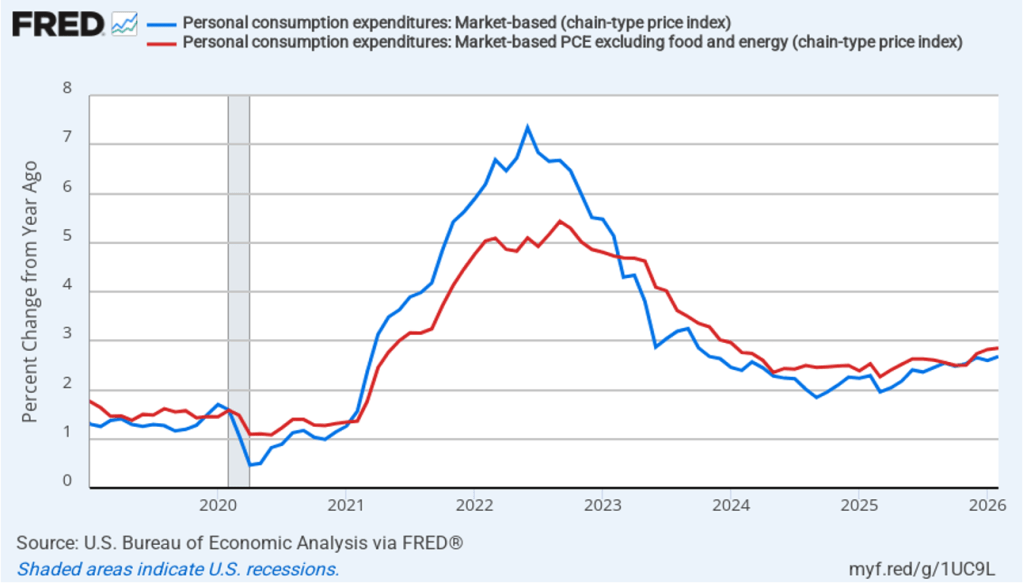
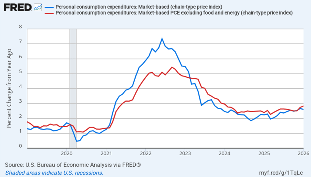
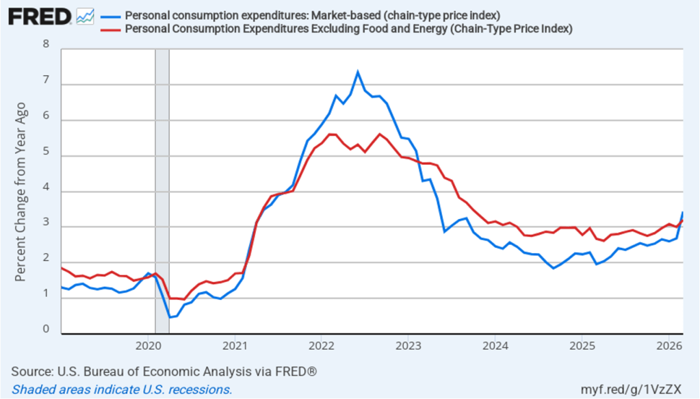
Fed Chair Jerome Powell has frequently mentioned that inflation in non-market services can skew PCE inflation. Non-market services are services whose prices the BEA imputes rather than measures directly. For instance, the BEA assumes that prices of financial services—such as brokerage fees—vary with the prices of financial assets. So that if stock prices rise, the prices of financial services included in the PCE price index also rise. Powell has argued that these imputed prices “don’t really tell us much about … tightness in the economy. They don’t really reflect that.” The following figure shows 12-month headline inflation (the blue line) and 12-month core inflation (the red line) for market-based PCE. (The BEA explains the market-based PCE measure here.)

Headline market-based PCE inflation was 3.4 percent in March, up from 2.9 percent in February. Core market-based PCE inflation was 3.1 percent in March, up from 2.9 percent in February. So, both market-based measures show inflation in March remaining well above the Fed’s 2 percent target.
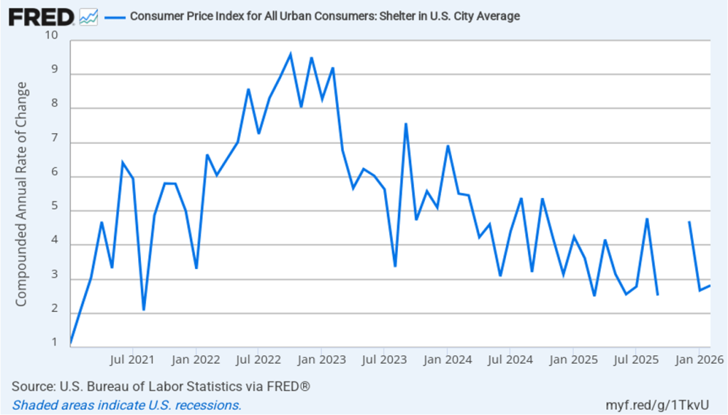
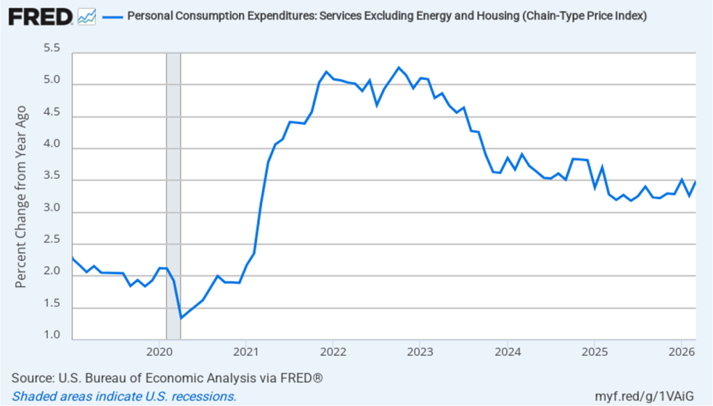
Increases in rent have been one driver of inflation. The following figure shows the 12-month change in service prices, excluding energy and housing prices. Inflation in service prices measured this way was 3.5 percent in March. One-month inflation (not shown) was even higher at 4.6 percent.
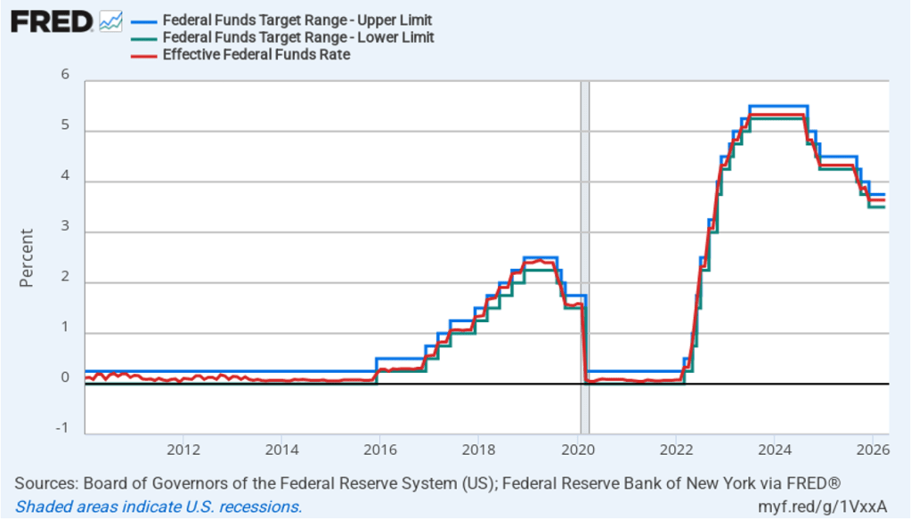
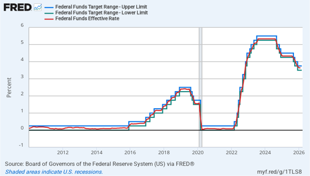
However measured, inflation is clearly running well above the Fed’s 2 percent target. Incoming Fed Chair Kevin Warsh is walking into a difficult situation. He’s likely to come under pressure from President Trump to convince his colleagues on the Federal Open Market Committee to cut the target for the federal funds rate. But it seems unlikely that a majority of the committee would be willing to cut the target with inflation remaining well above 2 percent. As we mentioned in yesterday’s post, investors who buy and sell federal funds futures contracts don’t expect that the target rate will be lowered before the committee’s meeting on December 14–15 2027.