

Photo of a meeting of the Federal Open Market Committee earlier this year from federalreserve.gov
What’s inflation? The answer seems easy: Inflation means that prices are rising …. but there are complications. When we experience inflation, does every price rise? If not, does it matter which prices or how many prices are rising? If a price rises one month and falls the next, is that still inflation?
We answer these questions in Macroeconomics, Chapter 19. As we discuss in that chapter, we measure inflation as the increase in the price level from one year to the next. We focus on the price level rather than on the prices of any particular goods or services because we want to know what is happening to a measure of average prices. Because we are looking at an average of prices, we would expect that when the economy experiences inflation, some prices will rise, but other prices may fall, and some prices may be unchanged.
Put another way, when we measure inflation, we are asking a macroeconomic question: Are there forces in the economy that are making an average of prices increase, and if so, by how much? When we look at individual prices, we are typically asking microeconomic questions: How much will an outbreak of avian flu increase the price of eggs? How much will a surge in constructing data centers increase the price of computer chips? Microeconomic developments do sometimes affect our inflation measures. For example, if conflict in the Middle East disrupts the flow of oil, raising oil prices, the effect may be large enough to increase the price level.

Image created by ChatGPT of oil tankers passing through the Strait of Hormuz
The two most closely watched measures of the price level are the consumer price index (CPI), which is compiled monthly by the Bureau of Labor Statistics (BLS), and the personal consumption expenditures (PCE) price index, which is compiled monthly by the Bureau of Economic Analysis (BEA). Economists and Federal Reserve policymakers prefer the PCE measure of the price level because it includes more goods and services than does the CPI. Each month’s release of CPI and PCE data can help answer three questions:
- How much inflation are consumers experiencing?
- How well is the Federal Reserve meeting its mandate from Congress to achieve price stability?
- How likely is inflation to persist?
The public’s strongly negative reaction to the Covid-era surge in inflation that began in the spring of 2021 made it clear that high inflation rates were an important political issue. The persistence of inflation rates above the Fed’s 2 percent annual target caused “affordability” to be an important issue in the 2026 midterm elections in the United States.
The CPI is designed to answer question 1. Although the inflation any individual household experiences will depend on the particular mix of goods and services consumed, the percentage change in the CPI provides a good measure of the inflation experienced by the typical household. The Fed answers question 2. using the percentage change in the PCE from the same month in the previous year. Fed policymakers have met the Congressional mandate for stable prices if the annual inflation rate as measured by the PCE is 2 percent or less. (Note that there is some debate whether 2 percent inflation represents “price stability” in the way Congress intended.)
Question 3. is the most difficult to answer. Future inflation rates depend partly on macroeconomic policy, particularly monetary policy, and on geopolitical developments, such as the likelihood that conflict in the Middle East will be resolved or will accelerate. But the details of how particular prices have been changing can also provide clues as to how persistent inflation is likely to be. Federal statistical agencies, economists, and policymakers make adjustments to the CPI and PCE with the aim of better identifying the underlying rate of inflation—that is, the movement in average prices after eliminating prices that may be increasing or decreasing for short-run, microeconomic reasons.
The best-known adjustments to the CPI and PCE are the core measures that exclude the prices of food and energy. The BLS began issuing a monthly measure of core CPI in 1977 and the BEA began issuing a monthly measure of core PCE in 2000, although it had been compiling a similar measure since 1974.

Image created by ChatGPT
The BLS explains why it began issuing data on core CPI:
“Food and especially energy have been more volatile in recent years than almost everything else in the CPI, and their sharp short-term movements up and down can dominate the movement of the All items [CPI] index, obscuring longer term underlying trends or important changes in other categories. … Inflation due largely to higher food or energy prices might have different policy implications than broader inflation.”
Fed policymakers have looked at a number of other ways to adjust the PCE to gauge the underlying inflation rate. For example, as we discuss in a recent blog post, Fed policymakers believe that inflation in non-market services can skew PCE inflation. Non-market services are services whose prices the BEA imputes rather than measures directly. For instance, the BEA assumes that prices of financial services—such as brokerage fees—vary with the prices of financial assets. So that if stock prices rise, the prices of financial services included in the PCE price index also rise. Former Fed Chair Jerome Powell has argued that these imputed prices “don’t really tell us much about … tightness in the economy. They don’t really reflect that.”

Image created by ChatGPT of Kevin Warsh testifying before the Senate Banking Committee
At his confirmation hearing before the Senate Banking Committee, Fed Chair Kevin Warsh, addressed the issue of determining the underlying inflation rate:
“What I’m most interested in is, what’s the underlying inflation rate? Not what’s the one time change in prices because of a change in geopolitics or a change in beef, but what’s the underlying generalized change in prices in the economy? … The measures I prefer are looking at things that are called trimmed averages, where we take out all of the tail risks, all of the one-off items, and we ask ourselves whether the generalized change in prices is having second order effects on the economy. … Some in the economics profession are increasingly looking to these median type measures ….”
As we’ve discussed in previous blog posts, two widely available measures of the type Warsh is referring to are:
- Trimmed-mean PCE inflation, which drops the 31 percent of goods and services with the highest inflation rates and the 24 percent of goods and services with the lowest inflation rates, and
- Median PCE inflation, which is calculated by listing the inflation rate in each individual good or service included in the PCE and identifying the inflation rate of the good or service that is in the middle of the list—that is, the inflation rate in the price of the good or service that has an equal number of higher and lower inflation rates.
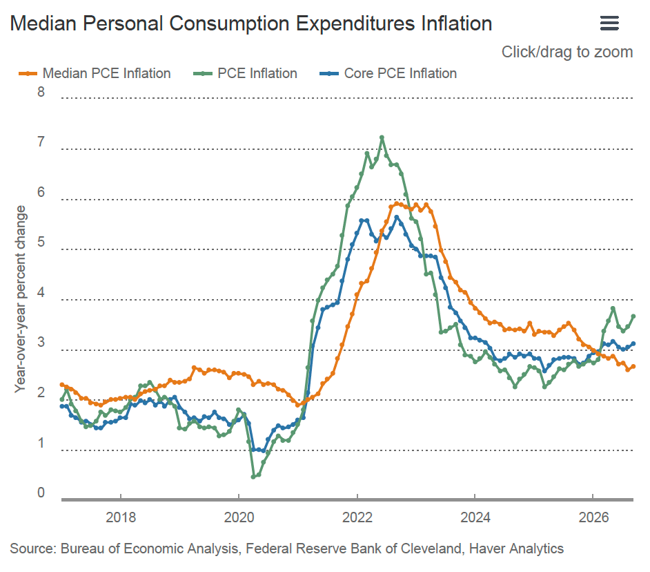
The following figure, from the website of the Federal Reserve Bank of Cleveland shows the relationship of headline PCE inflation (the green line), core PCE inflation (the blue line), and median PCE inflation (the brown line). Since March 2026, median inflation has been below both headline and core inflation, which may indicate that it is a better indicator of underlying inflation in the months since the conflict in the Middle East intensified.
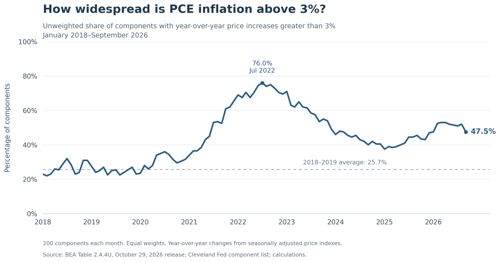
In an address in August at the Federal Reserve Bank of Kansas City’s economic policy symposium in Jackson Hole, Wyoming, Warsh discussed a less familiar indicator of underlying inflation: “To try to gauge underlying inflation, I find it instructive to disaggregate the 199 individual components of the PCE price measure. Over the past 12 months, 54 percent of goods and services in the PCE basket showed price increases above 3 percent. This is well below the post-pandemic highs of about 77 percent, but it remains well above the level of 32 percent in the two decades that preceded the pandemic.”

Image created by ChatGPT
The following figure shows for each month from January 2018 through September 2026, the fraction of PCE components that experienced price increases of greater than 3 percent. For instance, prices included in the PCE component “Personal computers/tablets and peripheral equipment” increased 9.7 percent from September 2025 to September 2026, while prices in the PCE component “Telephone and related communication equipment” decreased by 12.7 percent over the same period. The figure confirms Warsh’s statement: During 2018 and 2019, when headline PCE inflation was less than 2 percent in most months, 25.7 percent of PCE components experienced price increases of more than 3 percent, while in September 2026, 47.5 percent did.
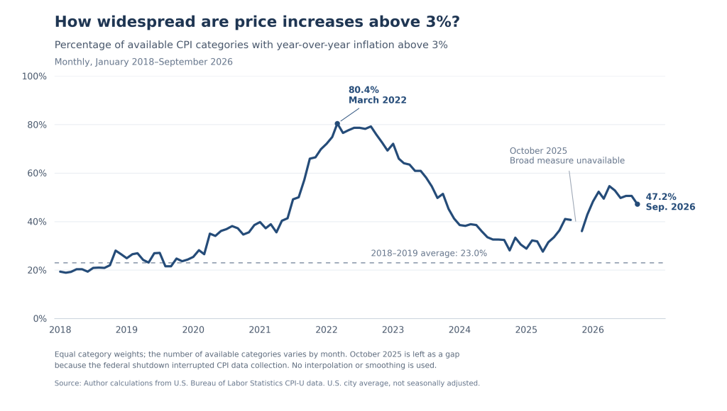
As the following figure shows, we get a similar result if we plot the same indicator for the CPI.
So, we have a number of ways of attempting to measure the underlying inflation rate. The reason, once again, why Fed policymakers are concerned about the underlying inflation rate rather than just the headline inflation rate is that monetary policy is better equipped to respond to movements in the underlying inflation rate than it is to respond to blips in the headline inflation rate that may be caused by transitory factors such as a sharp increase or decrease in energy prices.
Which measure of underlying inflation might be best? Here is ChatGPT’s (very long!) analysis.
ChatGPT on measures of underlying inflation
The three approaches answer different questions. A trimmed mean or median estimates a central rate of price increase after limiting the influence of unusually large increases and decreases. The percentage of categories rising more than 3% measures how widespread relatively rapid price increases are. My preference would be to use a trimmed mean and a median to assess the underlying inflation rate, and breadth to assess how generalized the pressure is.
The distinction matters because these measures can move in different directions without either being incorrectly calculated.
1. What each measure is trying to tell us
It helps to distinguish the measured change in the overall price index from indicators intended to extract a more persistent signal.
| Measure | Main question it answers | Principal strength | Principal limitation |
|---|---|---|---|
| Headline inflation | How much did the full price index increase? | Includes the entire consumption basket | Large movements in a few components can obscure the broader trend |
| Conventional core inflation | How much did prices excluding food and energy increase? | Simple, familiar, and consistently defined | Excludes some informative movements while retaining large movements elsewhere |
| Trimmed mean | What is the average increase among components in the middle of the price-change distribution? | Reduces sensitivity to extremes while preserving information about the size of central price changes | Results depend on trimming choices; excluded movements can contain useful information |
| Median | What price increase lies at the expenditure-weighted midpoint? | Strong protection against unusually large increases and decreases | Discards most information about the rest of the distribution |
| Share above 3% | How much of the basket—or how many categories—has inflation above a chosen threshold? | Makes the breadth of faster price increases easy to see | Does not measure how far above or below the threshold prices are rising |
The first conceptual caution is that an outlying price increase is not necessarily an error or a temporary disturbance. It can be a genuine, persistent change in a relative price. Removing its influence may help estimate the common inflation trend, but it also removes part of what consumers are paying.
A simple illustration
Suppose a hypothetical fixed-weight basket contains ten equally weighted categories. For illustration, calculate a trimmed mean by dropping the highest and lowest observations. All changes refer to the same period.
| Category price changes | Full-basket average | Trimmed mean | Median | Share above 3% |
|---|---|---|---|---|
| All ten rise 2% | 2% | 2% | 2% | 0% |
| Nine rise 2%; one rises 22% | 4% | 2% | 2% | 10% |
| Nine rise 4%; one falls 16% | 2% | 4% | 4% | 90% |
These are hypothetical calculations, not the precise construction of any published index.
The second row captures the usual argument for robust inflation measures: one exceptionally large increase raises the average even though most categories are rising moderately.
The third row is equally important. One exceptionally large decline can hold down headline inflation while most prices rise rapidly. Median and trimmed mean measures can therefore indicate more inflation pressure than the headline measure. Their purpose is to reduce the influence of both tails, rather than systematically produce a lower number.
2. Trimmed mean: a useful compromise between robustness and information
A trimmed mean ranks component price changes and removes a specified portion from each end of the distribution. It averages the remaining changes using their expenditure weights.
The precise implementation matters:
- The Dallas Fed trimmed mean PCE removes 24% of expenditure weight from the lower tail and 31% from the upper tail, retaining the middle 45%.
- The Cleveland Fed 16% trimmed mean CPI removes 8% of expenditure weight from each tail, retaining the middle 84%.
These are percentages of expenditure weight, not percentages of the number of category names. They are also quite different degrees of trimming, so “the trimmed mean” does not identify a unique estimator. Sources: Dallas methodologyand Cleveland methodology.
Advantages
It adapts to where the unusual movements occur. Conventional core inflation always excludes food and energy. A trimmed mean instead excludes whichever components have the most extreme changes that month. Food or energy can remain in the calculation when their changes are near the middle; a large movement elsewhere can be removed.
That is attractive because the economic reason for discounting a price movement is generally its usefulness as a signal of continuing inflation, rather than its membership in a permanently excluded category.
It retains information about the magnitude of many price changes. If numerous components in the retained middle rise from 2% to 4%, the trimmed mean responds to the size of those increases. It uses more of the distribution than a median and substantially more information about magnitude than a threshold count.
It limits offsetting distortions from the two tails. It can help identify whether low headline inflation reflects broadly moderate increases or a combination of substantial increases and a few very large declines.
Disadvantages
The trimming rule requires judgment. How much should be trimmed? Should the upper and lower tails be treated symmetrically? The answers depend partly on the distribution of relative-price changes and the statistical objective being pursued.
The Dallas proportions were selected using historical data. That provides an empirical foundation, but it does not guarantee that the same proportions will remain optimal in every subsequent inflation regime. Its asymmetric trimming also illustrates that a simple symmetric distribution of price changes cannot be taken for granted. Dallas methodology
It can remove economically important signals. An extreme increase may be the first sign of pressure that will spread to other categories. Alternatively, a sector may experience sustained inflation for several years. The trimming procedure classifies observations by their position in the distribution; it does not know whether the underlying cause is temporary, persistent, supply driven, or demand driven.
It cannot remove a shock merely because the shock is temporary. If a temporary common disturbance moves most prices, it moves the middle of the distribution too. A trimmed mean is robust to sufficiently concentrated extremes, not to every disturbance that policymakers might wish to look through.
My assessment is that a trimmed mean offers an appealing balance: it reduces the influence of exceptional observations while retaining meaningful information about the size of price changes across a substantial portion of spending.
3. Median inflation: greater resistance to extremes, greater loss of information
The published Cleveland Fed median measures are expenditure weighted. The components are ranked by their monthly price changes, and the median is the change at the 50th percentile of expenditure weight. It is not the inflation rate of the middle category in a list where every category receives one vote. See the median CPI and median PCE descriptions.
Advantages
The median is highly resistant to the size of extreme observations. If a component already in the upper tail rises 30% instead of 10%, that change generally has no effect on the median. The same applies to exceptionally large declines.
It provides a clear indication of movement in the center of the distribution. An increase in the median suggests that the distribution’s midpoint has shifted. It is less vulnerable to the interpretation that a rise in the average reflects only one or two extreme observations.
It avoids having to choose particular trimming percentages. Within the family of measures that focus on the middle of the distribution, the median has a transparent definition. That does not eliminate every methodological choice—component definitions, weights, and seasonal adjustment still matter—but it removes the choice between, say, an 8% and a 15% trim.
Disadvantages
A large amount of inflation pressure can occur away from the midpoint. Suppose 51% of expenditure weight has inflation of 2%, while the remaining 49% has inflation of 8%. In a simple fixed-weight calculation:
- Average inflation is 4.94%.
- Median inflation is 2%.
The median accurately describes the midpoint, but a policymaker would lose important information by looking only at that number.
It can also change abruptly. Reverse the weights to 49% at 2% and 51% at 8%, and the median jumps from 2% to 8%, even though average inflation rises only from 4.94% to 5.06%. Real data are more complicated, but the example shows why the median is not always a smooth measure of changes in the whole distribution.
Large expenditure categories can have considerable influence over which observation becomes the median. A large category occupies a wide interval of cumulative expenditure weight. Housing is particularly relevant. Cleveland revised its CPI methodology by dividing owners’ equivalent rent into four regional components to reduce the distortion that a single large OER component could create. This is a concrete example of how the level of aggregation affects a median. Cleveland methodology revision
The median need not have the same long-run average as headline inflation. Persistent relative-price trends and asymmetry in the distribution can create a systematic gap between the median and the mean. A Cleveland study found such a positive gap for median PCE in its historical sample. Consequently, a median reading of 2% is not automatically equivalent to aggregate PCE inflation being at the Fed’s 2% objective. Carroll and Verbrugge, 2019
I would use the median as a valuable check on whether the center is moving, while continuing to examine what is happening on either side of it.
4. The share above 3%: particularly useful for breadth, limited as an estimate of the inflation rate
For the unweighted version we have been considering, the calculation is:\[ \text{Breadth}_t = 100\times \frac{\text{number of categories with inflation above 3%}} {\text{number of categories observed}}. \]
An expenditure-weighted version instead adds up the spending shares of the categories above 3%. Those two calculations answer different questions.
Advantages
It directly addresses whether inflation is concentrated or widespread. An aggregate rate can be high because of a few exceptional increases or because of moderate increases across many categories. Breadth helps distinguish those situations.
Extreme observations have bounded influence. In an unweighted count, a category rising 50% contributes exactly as much as a category rising 4%. Each category can change the numerator by at most one. This makes the measure well suited to the particular question of how widely elevated inflation is distributed.
It can reveal changes that the median misses. Suppose the share above 3% rises from 20% to 45%. The median can remain below 3% throughout, yet the growing upper portion of the distribution may be informative. Breadth shows that development directly.
An unweighted count can reveal generalization across sectors without being dominated by the largest spending categories. That can be useful when each category is being treated as a separate signal about price-setting behavior. Equal weighting has a coherent purpose, even though it sacrifices a direct interpretation in terms of household spending.
Disadvantages
It throws away information about magnitude
Consider two hypothetical changes:
- Every category slows from 10% inflation to 4%. The share above 3% remains 100%, despite substantial disinflation.
- Every category moves from 2.9% to 3.1%. The share jumps from 0% to 100%, despite an increase of only 0.2 percentage point in every category.
The first example shows how breadth can miss major progress. The second shows how a hard threshold can exaggerate the apparent importance of a small movement.
This is why I would examine several thresholds or inflation-rate ranges, rather than place too much weight on whether a single 3% line has been crossed.
Weighting changes the economic interpretation
Suppose six small categories each account for 5% of spending and have inflation of 4%, while four larger categories each account for 17.5% of spending and have inflation of 1%.
Then:
| Statistic | Result |
|---|---|
| Percentage of categories above 3% | 60% |
| Percentage of expenditure weight above 3% | 30% |
| Expenditure-weighted median | 1% |
| Simple expenditure-weighted average | 1.9% |
The unweighted measure correctly reports that most categories have relatively rapid increases. It does not establish that most consumer spending is experiencing those increases.
Both versions are useful, provided their interpretation is explicit. For example, the Federal Reserve’s 2026 research on inflation breadth uses weighted shares of the CPI basket, as specified in its accessible figures. Those shares should not be compared directly with unweighted counts. Federal Reserve, Figures 2–3
The category classification can materially change the answer
If a category with inflation above 3% is divided into ten subcategories, each with the same inflation rate, its influence on an unweighted count increases even though nothing economic has changed.
A count therefore requires a consistent set of mutually exclusive categories at a reasonably stable level of detail. Counting both a broad category and its subcategories would effectively give some prices multiple votes.
Expenditure weighting avoids the particular problem of splitting an otherwise identical category: its total spending weight remains unchanged. But aggregation can still matter when subcategories have different inflation rates.
There is no universal “normal” share implied by the 2% target
The Fed’s objective concerns aggregate PCE inflation, not the inflation rate of every individual component.
For example, five equally weighted categories with inflation rates of:\[ -1\%,\quad 1\%,\quad 2\%,\quad 4\%,\quad 4\% \]
have average inflation of 2%, median inflation of 2%, and 40% of categories above 3%.
A substantial share above 3% can therefore coexist with aggregate inflation at target. What matters is how the share compares with an appropriate historical benchmark calculated in the same way. Warsh’s comparison with the prepandemic 32% is informative for that reason. But the historical average is an empirical benchmark, not an additional policy target.
5. Time horizon creates an especially important difference
There are two separate issues here.
Annual breadth can remain elevated after current price increases have stopped
Suppose many prices rise 4% once and then remain unchanged. Their year-over-year inflation rates will continue to exceed 3% for roughly a year after the increase.
A persistently high annual breadth measure could therefore reflect the continued presence of a past price-level adjustment in the calculation. It does not necessarily mean that comparable increases are continuing each month.
Shorter horizons help. Six-month annualized inflation responds more quickly than twelve-month inflation, while three-month inflation responds more quickly still. The tradeoff is greater sensitivity to short-run fluctuations and seasonal-adjustment issues.
Warsh’s 49% six-month share, compared with 54% over twelve months, is consistent with less widespread rapid increases in the more recent window. It does not, by itself, establish how much the aggregate inflation rate has slowed or where it will go next.
Published annual median inflation is not the median of annual component inflation
This is easy to overlook.
The published median and trimmed mean measures are constructed from monthly component price changes. Their longer-horizon rates accumulate those monthly robust changes. Taking the median across components first and then accumulating through time can produce a different answer from calculating annual inflation for every component first and then taking the median. Cleveland median PCE methodology; Dallas calculation code
A hypothetical example makes the difference clear:
- There are three equally weighted categories.
- Category A rises 4% in January and is otherwise unchanged.
- Category B is unchanged throughout the year.
- Category C rises 4% in July and is otherwise unchanged.
Every month, at least two categories have zero inflation. The monthly median is therefore always zero, and an index built by compounding those medians has zero annual inflation.
Yet at year-end, two of the three categories have risen 4%. The median of their annual inflation rates is 4%, and annual breadth above 3% is 66.7%.
This is one reason an annual breadth measure and a published annual median series can give different signals.
There is a useful mathematical connection when the weights, categories, and horizon are identical: if more than half the weight has inflation above 3%, the corresponding weighted median exceeds 3%. If Warsh’s 54% is an unweighted count, it implies that the unweighted median of those annual component changes exceeds 3%. It does not directly establish the value of the published expenditure-weighted median inflation series.
6. None of these measures identifies the cause or persistence of inflation by itself
The motivation for robust measures is strongest when unusually large component movements are mainly idiosyncratic disturbances around a more persistent common trend. But that is an economic interpretation of the distribution, rather than something established by trimming it.
A common supply shock can raise prices across many categories. Tariffs, for example, can affect final imported goods and domestic goods or services that use imported inputs. Federal Reserve research explicitly traces both channels across PCE categories. Minton and Somale, 2025
Consequently:
- High breadth does not establish that excess aggregate demand is the cause.
- A rise in the median does not establish that the shock will persist.
- A concentrated increase does not establish that its effects will soon disappear.
Breadth does help assess the claim that high inflation is confined to a few unusual categories. But distinguishing an ongoing inflation process from a price-level adjustment requires additional evidence about subsequent price changes, quantities, expectations, and the propagation of the original shock.
The same caution applies to smoothness. A smoother series is easier to interpret, but smoothness alone does not establish that it is a better forecast of future inflation.
7. What does the empirical evidence say?
The research supports using robust measures, but it does not identify a universal winner across objectives, samples, and forecast horizons.
Dallas Fed research finds a useful distinction between filtering and forecasting. Dolmas and Koenig’s 2019 comparison concludes that trimmed mean PCE is helpful for filtering transitory variation and has advantages as an estimate of underlying inflation. However, it does not clearly dominate conventional core PCE in real-time forecasts of headline PCE inflation. Those are different tests of usefulness. “Two Measures of Core Inflation: A Comparison”
Cleveland research finds that many trimming choices perform similarly. Meyer and Venkatu find a broad range of trimmed mean estimators with statistically indistinguishable performance, including the median. Their results support the usefulness of focusing on the middle of the distribution, while providing less support for claiming that one finely chosen trim is uniquely best. “Trimmed-Mean Inflation Statistics: Just Hit the One in the Middle”
Relative performance can change across periods. Carroll and Verbrugge’s comparison of median PCE, trimmed mean PCE, and conventional core measures finds that the performance of the median measures changed after the Great Recession. Their analysis emphasizes the role of changes in the asymmetry of the component-price distribution. “Behavior of a New Median PCE Measure: A Tale of Tails”
For breadth, an additional distinction is necessary. A measure can correlate closely with inflation in the same periodwithout being an especially good predictor of future inflation. The Federal Reserve’s 2026 breadth study estimates contemporaneous relationships and examines how those relationships changed after the pandemic. It does not establish that a count above 3% forecasts future inflation better than median or trimmed mean measures. Federal Reserve breadth study
These studies also cover different historical samples. Their results provide reasons to use the measures and evaluate them carefully, rather than guarantees about their ranking in the current environment.
8. How I would use them together
For assessing the inflation outlook relevant to Fed policy, I would give the measures distinct roles.
- Keep headline PCE as the outcome to explain and forecast. It is the index to which the Fed’s inflation objective applies. Conventional core PCE remains a useful, familiar comparison.
- Use trimmed mean PCE as a central estimate of underlying inflation, with median PCE as a check. My preference for the trimmed mean reflects its retention of more information about the magnitude of price changes. Agreement between it and the median increases confidence that the center of the distribution is moving. Disagreement is a reason to inspect the distribution.
- Use breadth to assess generalization. I would look at both category counts and expenditure-weighted shares, with consistent definitions and historical benchmarks. Examining several thresholds would reveal whether a change reflects a substantial distributional shift or many observations barely crossing 3%.
- Compare horizons and investigate the components driving disagreement. Twelve-month measures provide perspective; shorter-horizon measures help identify recent changes. The sector composition matters when deciding whether the signal reflects continuing pressure, an earlier adjustment, or an unusual pattern of offsetting increases and declines.
Applied to Warsh’s speech, the comparison of 54% with a prepandemic 32% is meaningful evidence that faster price growth was more widespread than in the benchmark period, assuming a consistent calculation. The fall from about 77% also documents a substantial reduction in breadth. Neither fact supplies a numerical estimate of the underlying inflation rate or determines its future persistence.
Breadth adds valuable distributional information to median and trimmed mean inflation. Its strongest role is as a complement: it tells us how far relatively rapid price increases extend across the basket, while the robust rate measures tell us more about the pace of price increases near the center.

