Image created by ChatGPT
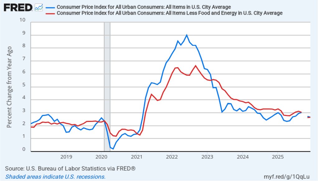
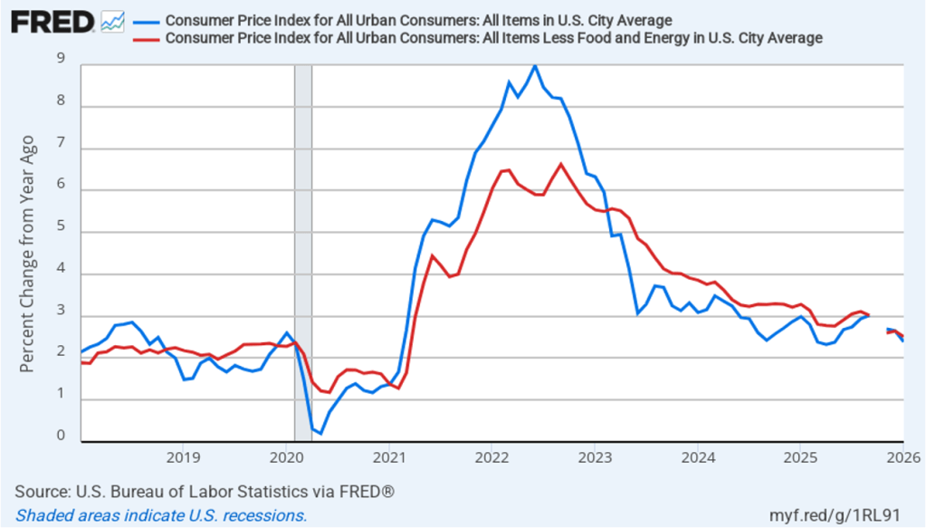
There was good news this morning on inflation. (Although maybe not quite good enough to justify the exuberance of the people in the AI-generated image above!) The Bureau of Labor Statistics (BLS) released its report on the consumer price index (CPI) for January. The following figure compares headline CPI inflation (the blue line) and core CPI inflation (the red line). Because of the effects of the federal government shutdown, the BLS didn’t report inflation rates for October or November, so both lines show gaps for those months. (Today’s report was delayed two days by the recent brief government shutdown.)
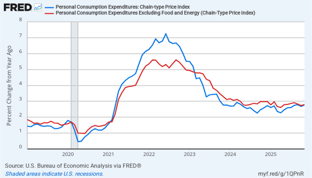
- The headline inflation rate, which is measured by the percentage change in the CPI from the same month in the previous year, was 2.4 percent in January, down from 2.7 percent in December.
- The core inflation rate, which excludes the prices of food and energy, was 2.5 percent in January, down from 2.6 percent in December.
Headline inflation was lower than the forecast of economists surveyed by FactSet, while core inflation was at the forecast rate.
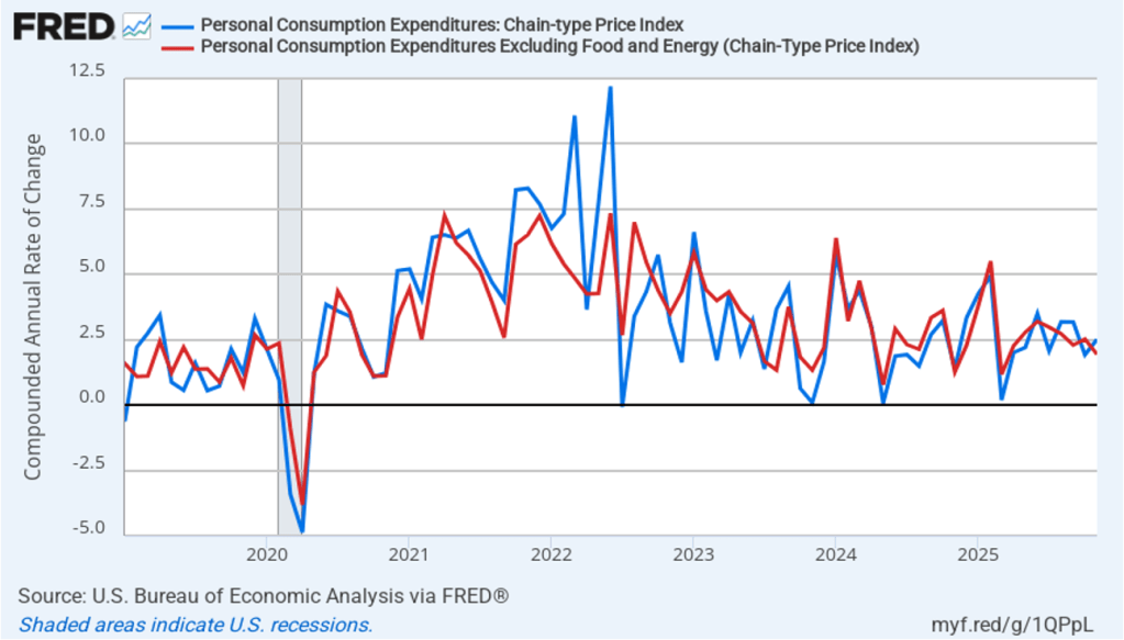
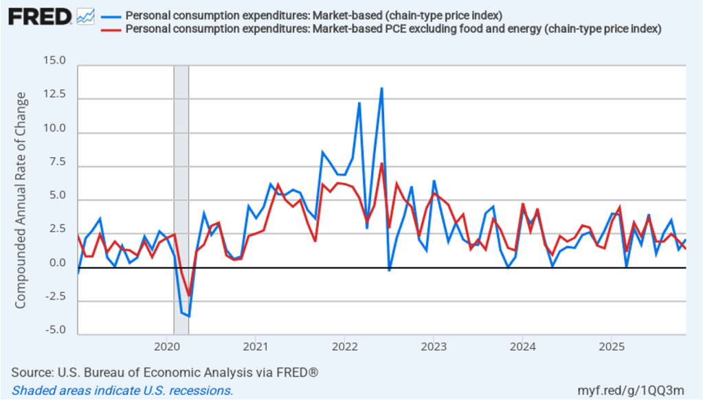
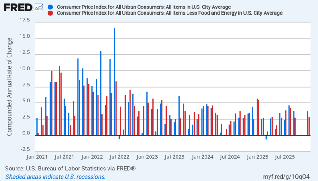
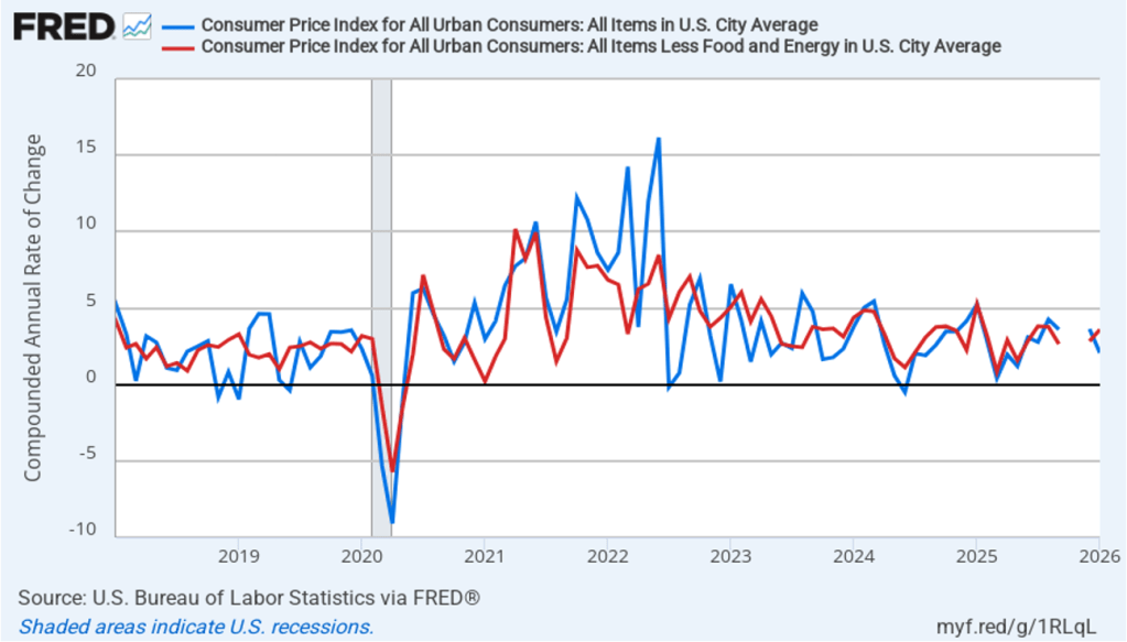
In the following figure, we look at the 1-month inflation rate for headline and core inflation—that is the annual inflation rate calculated by compounding the current month’s rate over an entire year. Calculated as the 1-month inflation rate, headline inflation (the blue line) was 2.1 percent in January, down from 3.6 percent in December. Core inflation (the red line) increased to 3.6 percent in January from 2.8 percent in December.
The 1-month and 12-month headline inflation rates are telling similar stories, with both measures indicating that the rate of price increase is running slightly above the Fed’s 2 percent inflation target. The 1-month core inflation rate shows inflation running well above the Fed’s target.
Of course, it’s important not to overinterpret the data from a single month. The figure shows that the 1-month inflation rate is particularly volatile. Also note that the Fed uses the personal consumption expenditures (PCE) price index, rather than the CPI, to evaluate whether it is hitting its 2 percent annual inflation target.
In recent months, there have been many media reports on how consumers are concerned about declining affordability. These concerns are thought to have contributed to Zohran Mamdani’s victory in New York City mayoral race. Affordability has no exact interpretation but typically means concern about inflation in goods and services that consumers buy frequently.
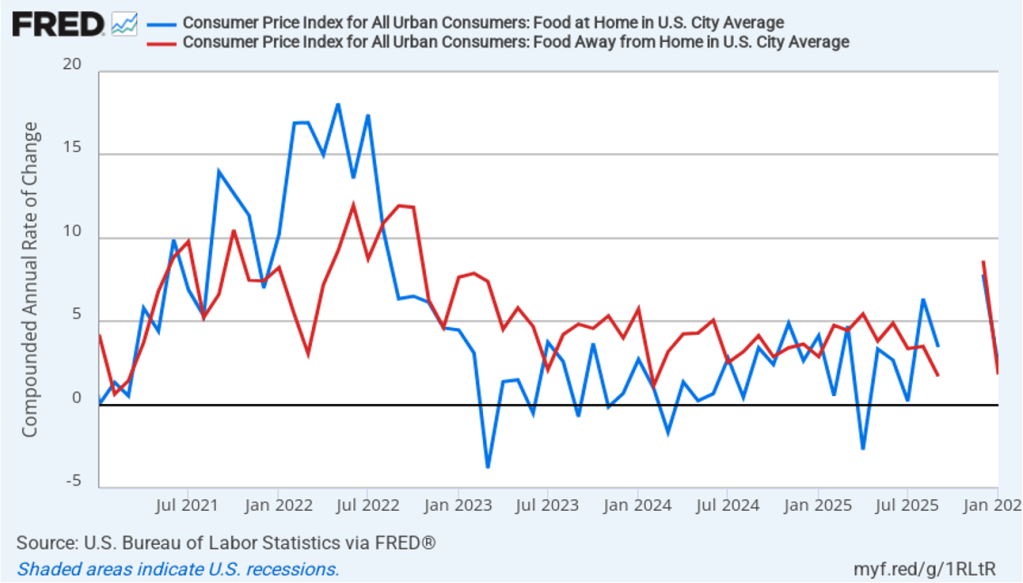
Many consumers seem worried about inflation in food prices. The following figure shows 1-month inflation in the CPI category “food at home” (the blue bar)—primarily food purchased at groceries stores—and the category “food away from home” (the red bar)—primarily food purchased at restaurants. Inflation in both measures fell in January from the very high leves of December. Food at home increased 2.3 percent in January, down sharply from up from 7.8 percent in December. Food away from home increased 1.8 percent in January, also down sharply from 8.7 percent in December. Again, 1-month inflation rates can be volatile, but the deceleration in inflation in food prices would be a welcome development if it can be sustained in future months.
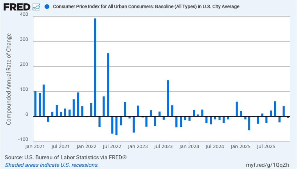
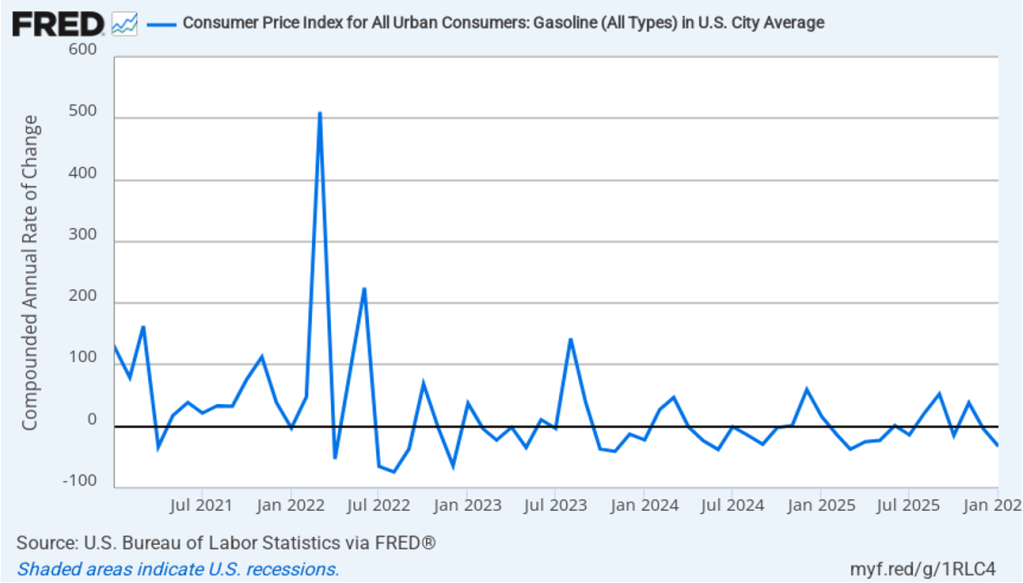
There was also good news in the falling price of gasoline. The following figure shows 1-month inflation in gasoline prices. In January the price of gasoline fell at an annual rate of 32.2 percent, after having fallen at an annual rate of 4.0 percent in December. As those values imply, 1-month inflation rates in gasoline are quite volatile.
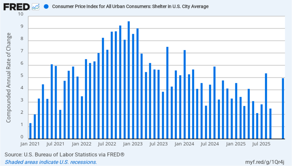
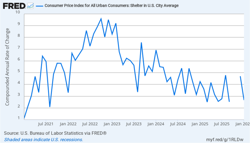
The affordability discussion has also focused on the cost of housing. The price of shelter in the CPI, as explained here, includes both rent paid for an apartment or a house and “owners’ equivalent rent of residences (OER),” which is an estimate of what a house (or apartment) would rent for if the owner were renting it out. OER is included in the CPI to account for the value of the services an owner receives from living in an apartment or house. The following figure shows 1-month inflation in shelter.
One-month inflation in shelter decreased to 2.7 percent in January from 4.7 in December, which is also good news if it can be sustained.
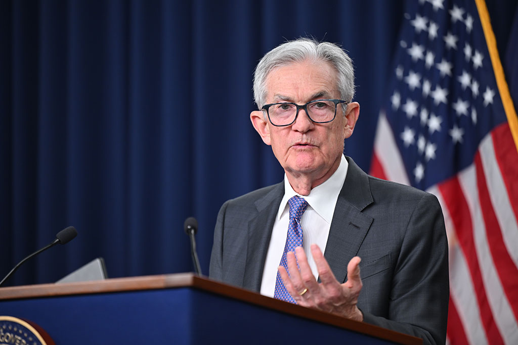
What effect have the tariffs that the Trump administration announced on April 2 had on inflation? (Note that many of the tariff increases announced on April 2 have since been reduced.) There has been a debate among policymakers and economists as to whether the full effects of tariff increases have already shown up in prices of final goods. In his press conference following the last meeing of the Fed’s Federal Open Market Committee (FOMC), Fed Chair Jerome Powell indicated that he believed that tariffs would cause further price increases later in the year:
“The U.S. economy has pushed right through [the tariff increases]. Partly that is—that the way that what was implemented was significantly less than what was announced at the beginning. In addition, other countries didn’t retaliate, and, in addition, a good part of it hasn’t been passed through to consumers yet. It’s being—it’s being taken by companies that stand between the consumer and the exporter.”
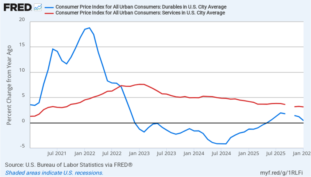
The following figure shows 12-month inflation in durable goods—such as furniture, appliances, and cars—which are likely to be affected directly by tariffs, and 12-month inflation in services, which are less likely to be affected by tariffs. In January, inflation in durable goods was 0.4 percent, down from 1.2 percent in December. Inflation in services was 3.2 percent in January, down slightly from 3.3 percent in December. So to this point, upward pressure on goods prices from the tariffs is not reflected in the most recent data.
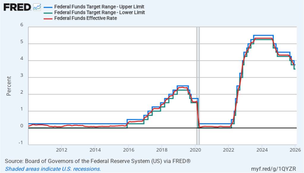
It’s unlikely that this inflation report will have much effect on the views of the members of the FOMC. The FOMC is unlikely to lower its target for the federal funds rate at its next meeting on March 17–18. The probability that investors in the federal funds futures market assign to the FOMC keeping its target rate unchanged at that meeting declined only slightly from 91.6 percent yesterday to 90.2 percent after the release of today’s inflation report.