HubbardOBrienEconomics.com Blog

As Expected, the FOMC Leaves Its Target for the Federal Funds Rate Unchanged

Federal Reserve Chair Jerome Powell at a press conference following a meeting of the FOMC (photo from federalreserve.gov)

Members of the Fed’s Federal Open Market Committee (FOMC) had signaled that the committee was likely to leave its target range for the federal funds rate unchanged at 4.25 percent to 4.50 percent at its meeting today (January 29), which, in fact, was what they did. As Fed Chair Jerome Powell put it at a press conference following the meeting:

“We see the risks to achieving our employment and inflation goals as being roughly in balance. And we are attentive to the risks on both sides of our mandate. … [W]e do not need to be in a hurry to adjust our policy stance.”

The next scheduled meeting of the FOMC is March 18-19. It seems likely that the committee will also keep its target rate constant at that meeting. Although at his press conference, Powell noted that “We’re not on any preset course.” And that “Policy is well-positioned to deal with the risks and uncertainties that we face in pursuing both sides of our dual mandate.” The statement the committee released after the meeting showed that the decision to leave the target rate unchanged was unanimous.

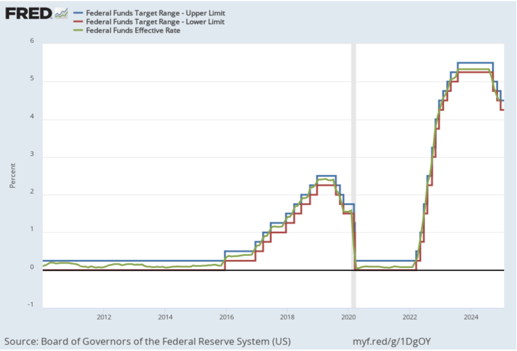
The following figure shows, for the period since January 2010, the upper bound (the blue line) and lower bound (the red line) for the FOMC’s target range for the federal funds rate and the actual values of the federal funds rate (the green line) during that time. Note that the Fed is successful in keeping the value of the federal funds rate in its target range.

A week ago, President Donald Trump in a statement to the World Economic Forum in Davos, Switzerland noted his intention to take actions to reduce oil prices. And that “with oil prices going down, I’ll demand that interest rates drop immediately.” As we noted in this recent post about Fed Governor Michael Barr stepping down as Fed Vice Chair for Supervision, there are indications that the Trump administration may attempt to influence Fed monetary policy.

In his press conference, Powell was asked about the president’s statement and responded that he had “No comment whatever on what the president said.” When asked whether the president had spoken to him about the need to lower interest rates, Powell said that he “had no contact” with the president. Powell stated in response to another question that “I’m not going to—I’m not going to react or discuss anything that any elected politician might say ….”

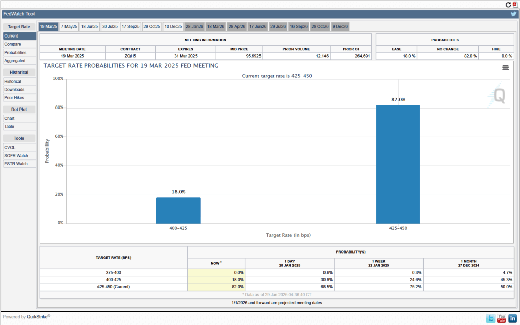
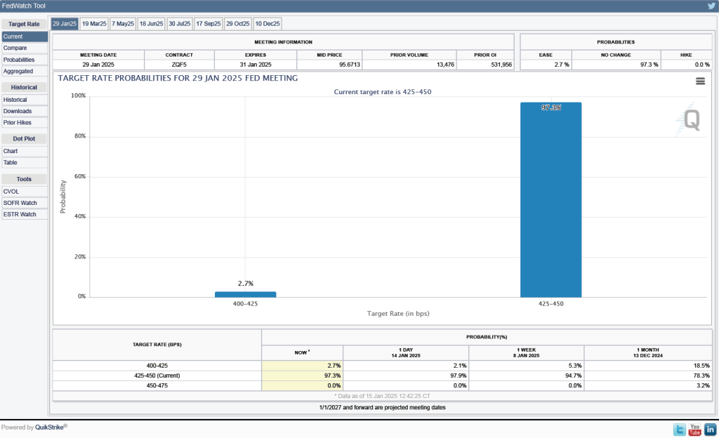
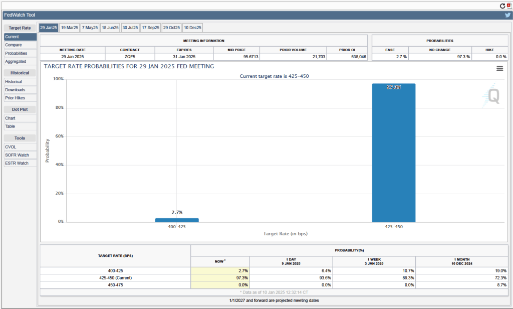
As we noted earlier, it seems likely that the FOMC will leave its target for the federal funds rate unchanged at its meeting on March 18-19. One indication of expectations of future rate cuts comes from investors who buy and sell federal funds futures contracts. (We discuss the futures market for federal funds in this blog post.) As shown in the following figure, today these investors assign a probability of 82.0 percent to the FOMC keeping its target range for the federal funds rate unchanged at the current range of 4.25 percent to 4.50 percent at the March meeting. Investors assign a probability of only 18.0 percent to the committee cutting its target range by 25 basis points at that meeting.

DeepSeek, Nvidia, and the Effect of New Information on Stock Prices

At the close of stock trading on Friday, January 24 at 4 pm EST, Nvidia’s stock had a price of $142.62 per share. When trading reopened at 9:30 am on Monday, January 27, Nvidia’s stock price plunged to $127.51. The total value of all Nvidia’s stock (the firm’s market capitalization or market cap) dropped by $589 billion—the largest one day drop in market cap in history. The following figure from the Wall Street Journal shows movements in Nvidia’s stock price over the past six months.

What happened to cause should a dramatic decline in Nvidia’s stock price? As we discuss in Macroeconomics, Chapter 6 (Economics, Chapter 8, and Money, Banking, and the Financial System, Chapter 6), Nividia’s price of $142.62 at the close of trading on January 24—like the price of any publicly traded stock—reflected all the information available to investors about the company. For the company’s stock to have declined so sharply at the beginning of the next trading day, important new information must have become available—which is exactly what happened.

As we discussed in this blog post from last October, Nvidia has been very successful in producing state-of-the-art computer chips that power the most advanced generative artificial intelligence (AI) software. Even after Monday’s plunge in the value of its stock, Nvidia still had a market cap of nearly $3.5 trillion at the end of the day. It wasn’t news that DeepSeek, a Chinese AI company had produced AI software called R1 that was similar to ChatGTP and other AI software produced by U.S. companies. The news was that R1—the latest version of the software is called V3—appeared to be comparable in many ways to the AI software produced by U.S. firms, but had been produced by DeepSeek despite not using the state-of-the-art Nvidia chips used in those AI programs.

The Biden administration had barred export to China of the newest Navidia chips to keep Chinese firms from surging ahead of U.S. firms in developing AI. DeepSeek claimed to have developed its software using less advanced chips and have trained its software at a much lower cost than U.S. firms have been incurring to train their software. (“Training” refers to the process by which engineers teach software to be able to accurately solve problems and answer questions.) Because DeepSeek’s costs are lower, the company charges less than U.S. AI firms do to use its computer infrastructure to handle business tasks like responding to consumer inquiries.

If the claims regarding DeepSeek’s software are accurate, then AI firms may no longer require the latest Nvidia chips and may be forced to reduce the prices they can charge firms for licensing their software. The demand for electricity generation may also decline if it turns out that the demand for AI data centers, which use very large amounts of power, will be lower than expected.

But on Monday it wasn’t yet clear whether the claims being made about DeepSeek’s software were accurate. Some industry observers speculated that, despite the U.S. prohibition on exporting the latest Nvidia chips to China, DeepSeek had managed to obtain them but was reluctant to admit that it had. There were also questions about whether DeepSeek had actually spent as little as it claimed in training its software.

What happens to the price of Nvidia’s stock during the rest of the week will indicate how investors are evaluating the claims DeepSeek made about its AI software.

Glenn on How the Trump Administration Can Hit Its Growth Target

Treasury Secretary nominee Scott Bessent. (Photo from Progect Syndicate.)

By setting an ambitious 3% growth target, U.S. Treasury Secretary nominee Scott Bessent has provided the Trump administration a North Star to follow in devising its economic policies. The task now is to focus on productivity growth and avoiding any unforced errors that would threaten output.

U.S. Treasury Secretary nominee Scott Bessent is right to emphasize faster economic growth as a touchstone of Donald Trump’s second presidency. More robust growth not only implies higher incomes and living standards—surely the basic objective of economic policy—but also can reduce America’s yawning federal budget deficit and debt-to-GDP ratio, and ease the sometimes difficult trade-offs across defense, social, and education and research spending.

But faster growth must be more than just a wish. Achieving it calls for a carefully constructed agenda, based on a recognition of the channels through which economic policies can raise or reduce output. While a pro-investment tax policy might boost capital accumulation, productivity, and GDP, higher interest rates from deficit-financed tax or spending changes might have the opposite effect. Similarly, since growth in hours worked is a component of growth in output or GDP, the new administration should avoid anti-work policies that hinder full labor-force participation, as well as sudden adverse changes to legal immigration.

While recognizing that some policy shifts that increase output might adversely affect other areas of social interest (such as the distribution of income) or even national security, policymakers should focus squarely on increasing productivity. The three pillars of any productivity policy are support for research, investment-friendly tax provisions, and more efficient regulation.

Ideas drive prospects in modern economies. Basic research in the sciences, engineering, and medicine power the innovation that advances technology, improvements in business organization, and gains in health and well-being. It makes perfect sense for the federal government to support such research. Since private firms cannot appropriate all the gains from their own outlays for basic research, they have less of an incentive to invest in it. Moreover, government support in this area produces valuable spillovers, as demonstrated by the earlier Defense Department research expenditures that became catalysts for today’s digital revolution.

This being the case, cuts in federal support for basic research are inconsistent with a growth agenda. Still, policymakers should review how research funds are distributed to ensure scientific merit, and they should encourage a healthy dose of risk-taking on newer ideas and researchers.

In addition to encouraging commercialization of spillovers from basic research and defense programs, federal support for applied research centers around the country would accelerate the dissemination of new productivity-enhancing technologies and ideas. Such centers also tend to distribute the economy’s prosperity more widely, by making new ideas broadly accessible—as agricultural- and manufacturing-extension services have done historically.

To address the second pillar of productivity growth, the administration should seek to extend the pro-investment provisions of the Tax Cuts and Jobs Act that Trump signed into law in 2017. While the TCJA’s lower tax rates on corporate profits remain in place, the expensing of business investment – a potent tool for boosting capital accumulation, productivity, and incomes – was set to be phased out over the 2023-26 period. This provision could be restored and made permanent by reducing spending on credits under the Inflation Reduction Act, or by rolling back the spending – such as $175 billion to forgive student loans – associated with outgoing President Joe Biden’s executive orders.

If the new administration wanted to go further with tax policy, it could build on the 2016 House Republican blueprint for tax reform that shifted the business tax regime from an income tax to a cashflow tax. By permitting immediate expensing of investment, but not interest deductions for nonfinancial firms, this reform would stimulate investment and growth, remove tax incentives that favor debt over equity, and simplify the tax system.

That brings us to the third pillar of a successful growth strategy: efficient regulation. The issue is not “more” versus “less.” What really matters for growth is how changes in regulation can improve the prospects for growth through innovation, investment, and capital allocation, while focusing on trade-offs in risks. Those shaping the agenda should start with basic questions like: Why can’t we build better infrastructure faster? Why can’t capital markets and bank lending be nimbler? Not only do such questions identify a specific goal; they also require one to identify trade-offs.

Fortunately, financial regulation under the new administration is likely to improve capital allocation and the prospects for growth, given the leadership appointments already announced at the Securities and Exchange Commission and the Federal Reserve. But policymakers also will need to improve the climate for building infrastructure and enhancing the country’s electricity grids to support the data centers needed for generative artificial intelligence. This will require a sharper focus on cost-benefit analysis at the federal level, as well as better coordination with state and local authorities on permitting. Using federal financial support programs as carrots or sticks can be part of such a strategy.

Bessent’s emphasis on economic growth is spot on. By setting an ambitious 3% target for annual growth, he has provided the new administration a North Star to follow in devising its economic policies.

This commentary first appeared on Project Syndicate.

1/17/25 Podcast – Authors Glenn Hubbard & Tony O’Brien discuss the pros/cons of tariffs and the impact of AI on the economy.

Welcome to the first podcast for the Spring 2025 semester from the Hubbard/O’Brien Economics author team. Check back for Blog updates & future podcasts which will happen every few weeks throughout the semester.

Join authors Glenn Hubbard & Tony O’Brien as they offer thoughts on tariffs in advance of the beginning of the new administration. They discuss the positive and negative impacts of tariffs -and some of the intended consequences. They also look at the AI landscape and how its reshaping the US economy. Is AI responsible for recent increased productivity – or maybe just the impact of other factors. It should be looked at closely as AI becomes more ingrained in our economy.

https://on.soundcloud.com/8ePL8SkHeSZGwEbm8

Did Stephen King Stumble into One of Our “Pitfalls in Decision Making”?

The cover of Steven King’s novel The Stand. (Image from amazon.com)

In Microeconomics, Chapter 10, we have a section on “Pitfalls in Decision Making.” One of those pitfalls is the failure to ignore sunk costs. A sunk cost is one that has already been paid and cannot be recovered.

In his book On Writing: A Memoir of the Craft, King discusses his writing of The Stand (a book he describes as “the one my longtime readers still seem to like the best.”) At one point he had had trouble finishing the manuscript and was considering whether to stop working on the novel:

“If I’d had two or even three hundred pages of single-spaced manuscript instead of more than five hundred, I think I would have abandoned The Stand and gone on to something else—God knows I had done it before. But five hundred pages was too great an investment, both in time and in creative energy; I found it impossible to let go.”

King seems to have committed the error of ignoring sunk costs. The time and creative energy he had put into writing the 500 pages were sunk—whether he abandoned the manuscript or continued writing until the book was finished, he couldn’t get back the time and energy he had expanded on writing the first five hundred pages. That he had already written 300 pages or 500 pages wasn’t relevant to his decision because if a cost is sunk it doesn’t matter for decision making whether the cost is large or small.

Is it relevant in assessing King’s decision that in the end he did finish The Stand, the novel sold well—earning King substantial royalties—and his fans greatly admire the novel? Not directly because only with hindsight do we know that The Stand was successful. In deciding whether to finish the manuscript, King shouldn’t have worried about the cost of the time and energy he had already spent writing it. Instead, King should have compared the expected marginal cost of finishing the manuscript with the expected marginal benefit from completing the book. Note that the expected marginal benefit could include not only the royalty earnings from sales of the books, but also the additional appreciation he received from his fans for writing what turned out to be their favorite novel.

When King paused working on the manuscript after having written 500 pages, the marginal cost of finishing was the opportunity cost of not being able to spend those hours and creative energy writing a different book. Given the success of The Stand, the marginal benefit to King from completing the manuscript was almost certainly greater than the marginal cost. So, completing the manuscript was the correct decision, even if he made it for the wrong reason!

The Southern California Wildfires and Problems in the Insurance Industry

Fire damage in the Pacific Palisades. (Photo from Reuters via the Wall Street Journal)

As of January 15, the series of devastating wildfires in Southern California have killed at least 25 people and destroyed billions of dollars’ worth of homes and businesses. Adding to the tragedy is the fact that many homeowners aren’t fully insured against the damage. As a result, they lack the necessary funds to rebuild their homes. Unfortunately for these people, the market for fire insurance in California hasn’t been working well.

In the United States, regulation of property and casualty insurance occurs at the state level with regulations differing substantially across states. In California, insurance companies face an unusually long regulatory process to receive permission to increase the premiums they charge. The delays in raising premiums have contributed to companies not renewing property insurance policies in some areas, such as those prone to wildfires. In these areas, the payouts the companies expect to make have been higher than the premiums that California regulators have allowed companies to charge policyholders.

The wildfires have ravaged the Pacific Palisades neighborhood of Los Angeles . Although housing prices in the neighborhood are among the highest in the country, an analysis by the Reuters news agency showed that: “Measured against home values, insurance costs are cheaper in the Palisades than in 97% of U.S. postal codes …” For example, the median insurance premium in the Pacific Palisades was “less than residents paid in Glencoe, Illinois, an upscale suburb of Chicago where homes are two-thirds cheaper and the risk of wildfire is minimal.”

Catastrophe modeling is a way of statistically forecasting the probability of events—such as floods or wildfires—occurring that would sharply increase claims by policyholders. Regulations had barred insurance companies from using catastrophe modeling to justify increases in premiums. (State regulators lifted the prohibition on the use of catastrophe modeling shortly before the fires.) These restrictions made it more difficult for companies to charge risk-based premiums, which are based on the probability that a policyholder will file a claim.

Insurance markets can experience adverse selection problems because the people most eager to buy insurance are those with highest probability of requiring an insurance payout. Insurance companies attempt to reduce adverse selection problems by, among other things, charging risk-based premiums. Limiting the ability of insurance companies to charge risk-based premiums increased the adverse selection problems the companies face. To cope with the problem of companies not renewing policies, regulators began requiring companies to renew policies in some Zip codes, particularly those that were in or near areas that had experienced wildfires. This policy further increased adverse selection.

By 2023, some insurers, including State Farm and Allstate—which are two of the largest property insurers in the United States—had decided that they were unlikely to be able cover their costs from offering property insurance policies in California and stopped writing policies in the state. Policyholders who are unable to obtain a policy from a private insurance company typically buy a policy offered through the Fair Access to Insurance Requirements (FAIR) Plan. The FAIR Plan is sponsored by the state government, although operated by private insurance companies. The premiums charged for a FAIR Plan policy are significantly higher than the premiums charged for a traditional policy. Despite the higher premiums, the number of FAIR Plan policies doubled between 2020 and 2025, reaching nearly 500,000.

The FAIR Plan lacks sufficient funds to pay the claims from policyholders who had lost their homes or businesses in the Southern California wildfires. To cover the deficit, the FAIR Plan will assess private insurance companies, who, in turn, will raise premiums charged to their other policyholders. In this way, some of the costs from the wildfires will be borne by all property insurance policyholders in California, even if they live far from the areas affected by the wildfires.

We discuss moral hazard in insurance markets in Microeconomics and Economics, Chapter 7 (and in Money, Banking, and the Financial System, Chapter 11). In general, moral hazard refers to actions people take after they have entered into a transaction that make the other party to the transaction worse off. Moral hazard in insurance markets occurs when people change their behavior after becoming insured. The way that the insurance market is regulated in California and, in particular, the way that the FAIR Plan is administered increases moral hazard because people who own homes or businesses in areas with a greater risk of damage from wildfires don’t pay premiums that fully reflect that greater risk. In other words, more people live in fire prone areas in California than would do so if the premiums on their insurance policies fully reflected the probability of their making a claim.

Whether, following the wildfires, the California legislature will change the regulations governing the insurance market is unclear at this point. As an insurance agent quoted by the Wall Street Journal put it: “We are in uncharted territory.”

Headline CPI Inflation Is Higher in December but Core Inflation Is Lower than Expected

Image generated by GTP-4o illustrating inflation

On January 15, the Bureau of Labor Statistics (BLS) released its monthly report on the consumer price index (CPI). The following figure compares headline inflation (the blue line) and core inflation (the green line).

The headline inflation rate, which is measured by the percentage change in the CPI from the same month in the previous month, was 2.9 percent in December—up from 2.7 percent in November.
The core inflation rate, which excludes the prices of food and energy, was 3.2 percent in December—down from 3.3 percent in November.

Headline inflation was slightly above and core inflation was slightly below what economists surveyed had expected.

In the following figure, we look at the 1-month inflation rate for headline and core inflation—that is the annual inflation rate calculated by compounding the current month’s rate over an entire year. Calculated as the 1-month inflation rate, headline inflation (the blue line) jumped from 3.8 percent in November to 4.8 percent in December. Core inflation (the green line) decreased from 3.8 percent in November to 2.7 percent in December.

Overall, considering 1-month and 12-month inflation together, the most favorable news is the low value of the 1-month core inflation rate. The most concerning news is a sharp increase in 1-month headline inflation, which brought that measure to its highest reading since February 2024. On balance, this month’s CPI report doesn’t do much to challenge the conclusion of other recent inflation reports that progress on lowering inflation has slowed or, possibly, stalled. So, the probability of a “no landing” outcome, with inflation remaining above the Fed’s target for an indefinite period, seems to have at least slightly increased.

Of course, it’s important not to overinterpret the data from a single month. The figure shows that 1-month inflation is particularly volatile. Also note that the Fed uses the personal consumption expenditures (PCE) price index, rather than the CPI, to evaluate whether it is hitting its 2 percent annual inflation target.

As we’ve discussed in previous blog posts, Federal Reserve Chair Jerome Powell and his colleagues on the Fed’s policymaking Federal Open Market Committee (FOMC) have been closely following inflation in the price of shelter. The price of “shelter” in the CPI, as explained here, includes both rent paid for an apartment or a house and “owners’ equivalent rent of residences (OER),” which is an estimate of what a house (or apartment) would rent for if the owner were renting it out. OER is included in the CPI to account for the value of the services an owner receives from living in an apartment or house.

As the following figure shows, inflation in the price of shelter has been a significant contributor to headline inflation. The blue line shows 12-month inflation in shelter, and the red line shows 1-month inflation in shelter. Twelve-month inflation in shelter has been declining since the spring of 2023, but in December it was still high at 4.6 percent. One-month inflation in shelter—which is much more volatile than 12-month inflation in shelter—fell from 4.1 percent in November to 3.1 percent in December.

To better estimate of the underlying trend in inflation, some economists look at median inflation and trimmed mean inflation.

Median inflation is calculated by economists at the Federal Reserve Bank of Cleveland and Ohio State University. If we listed the inflation rate in each individual good or service in the CPI, median inflation is the inflation rate of the good or service that is in the middle of the list—that is, the inflation rate in the price of the good or service that has an equal number of higher and lower inflation rates.
Trimmed mean inflation drops the 8 percent of goods and services with the highest inflation rates and the 8 percent of goods and services with the lowest inflation rates.

The following figure shows that 12-month median inflation (the red line) declined slightly from 3.9 percent in November to 3.8 percent in December. Twelve-month trimmed mean inflation (the blue line) was unchanged at 3.2 percent for the fifth month in a row.

The following figure shows 1-month median and trimmed mean inflation. One-month median inflation rose from 2.8 percent in November to 3.6 percent in December. One-month trimmed mean inflation fell slightly from 3.3 percent in November to 3.2 percent in December. These data provide confirmation that (1) CPI inflation at this point is likely running higher than a rate that would be consistent with the Fed achieving its inflation target, and (2) that progress toward the target has slowed.

What are the implications of this CPI report for the actions the FOMC may take at its next meeting on January 28-29? The stock market rendered a quick verdict, as the following figure from the Wall Street Journal shows. As soon as the market opened on Wednesday morning, all three of the most widely followed stock market indexes jumped—as indicated by the vertical segments in the figure. Investors seem to be focusing on core CPI inflation being lower than expected, which should increase the probability that the FOMC will cut its target for the federal funds rate at either its March or May meeting. Lower inflation and lower interest rates would be good news for stock prices.

Investors who buy and sell federal funds futures contracts still do not expect that the FOMC will cut its target for the federal funds rate at its next meeting, as indicated by the following figure. (We discuss the futures market for federal funds in this blog post.) Today, investors assign a probability of 93.7 percent to the FOMC leaving its target range for the federal funds rate unchanged at 4.25 percent to 4.50 percent at its January 28-29 meeting, and a probability of only 2.7 percent to the committee cutting its target range by 0.25 percentage point (25 basis points).

Unexpectedly Strong Jobs Report

Last September the Federal Reserve’s policymaking Federal Open Market Committee (FOMC) cut its target for the federal funds rate by 0.50 percentage point (50 basis points. Many economists and policymakers expected the FOMC to continue cutting its federal funds rate target at meetings through 2025. (We discussed the September target cut in this blog post.) The FOMC cut its target by 25 basis points at both its November and December 2024 meetings. But by the December meeting, it had become clear that the inflation rate was not falling as quickly to the Fed’s 2 percent target as the committee members had hoped. As FOMC’s staff economists put it, there had been “upward surprises” in inflation data. According to the minutes of the December meeting, several members of the committee believed that “upside risks to the inflation outlook had increased.”

As a result, it seemed likely that the FOMC would leave its target for the federal funds rate unchanged at its next meeting on January 28-29. This conclusion was reinforced this morning (January 10) when the Bureau of Labor Statistics (BLS) released its “Employment Situation” report (often called the “jobs report”) for December. The report indicates that the labor market is stronger than expected.

Economists who had been surveyed by the Wall Street Journal had forecast that payroll employment, as reported in the establishment survey, would increase by 155,000. The BLS reported that payroll employment in December had increased by 256,000, well above expectations. The unemployment rate—which is calculated from data in the household survey—was 4.1 percent, down slightly from 4.2 percent in November. The following figure, taken from the BLS report, shows the net changes in employment for each month during the past two years.

As the following figure shows, the net change in jobs from the household survey moves much more erratically than does the net change in jobs from the establishment survey. The net change in jobs as measured by the household survey for December also showed a strong increase of 478,000 jobs following a decline of 273,000 jobs in November. In any particular month, the story told by the two surveys can be inconsistent with employment increasing in one survey while falling in the other. But in December the two surveys were sending the same signal of rapid employment growth. (In this blog post, we discuss the differences between the employment estimates in the household survey and the employment estimates in the establishment survey.)

The employment-population ratio for prime age workers—those aged 25 to 54—also increased, as shown in the following figure, to 80.5 percent in December from 80.4 percent in November. Although the employment-population is below its recent high of 80.9 percent, it remains high relative to levels seen since 2001.

As the following figure shows, the unemployment rate, which is also reported in the household survey, decreased slightly to 4.1 percent in December from 4.2 percent in November. The unemployment rate has been remarkably stable over the past two years, varying only 0.2 percentage point above or below 4.0 percent.

The establishment survey also includes data on average hourly earnings (AHE). As we noted in this post, many economists and policymakers believe the employment cost index (ECI) is a better measure of wage pressures in the economy than is the AHE. The AHE does have the important advantage that it is available monthly, whereas the ECI is only available quarterly. The following figure shows the percentage change in the AHE from the same month in the previous year. The AHE increased 3.9 percent in December, down slightly from 4.0 percent in November.

The following figure shows wage inflation calculated by compounding the current month’s rate over an entire year. (The figure above shows what is sometimes called 12-month wage inflation, whereas this figure shows 1-month wage inflation.) One-month wage inflation is much more volatile than 12-month wage inflation—note the very large swings in 1-month wage inflation in April and May 2020 during the business closures caused by the Covid pandemic. The December 1-month rate of wage inflation was 3.4 percent, a decline from the 4.9 percent rate in November. Whether measured as a 12-month increase or as a 1-month increase, AHE is still increasing somewhat more rapidly than is consistent with the Fed achieving its 2 percent target rate of price inflation.

Given these data from the jobs report, it seems unlikely that the FOMC will reduce its target range for the federal funds rate at its next meeting. One indication of expectations of future rate cuts comes from investors who buy and sell federal funds futures contracts. (We discuss the futures market for federal funds in this blog post.) As shown in the following figure, today these investors assign a probability of 97.3 percent to the FOMC keeping its target range for the federal funds rate unchanged at the current range of 4.25 percent to 4.50 percent, at its next meeting. Investors assign a probability of only 2.7 percent of the committee cutting its target range by 25 basis points at that meeting.

As the following figure shows, investors also expect the FOMC to keep its target range unchanged at its meeting on March 18-19, although there is greater uncertainty. Investors assign:

A 74.0 percent probability that the FOMC keeps its target range for the federal funds rate unchanged
A 25.4 percent probability that the committee cuts its target range by 25 basis points
A 0.6 percent probability that the committee cuts its target range by 50 basis points

Yesterday at the Fed Something Happened That Was Unusual … or Was It?

Photo of Michael Barr from federalreserve.gov

President-elect Donald Trump has stated that he believes that presidents should have more say in monetary policy. There had been some speculation that once in office Trump would try to replace Federal Reserve Chair Jerome Powell, although Trump later indicated that he would not attempt to replace Powell until Powell’s term as chair ends in May 2026. Can the president remove the Fed Chair or another member of the Board of Governors? The relevant section of the Federal Reserve Act States that: “each member [of the Board of Governors] shall hold office for a term of fourteen years from the expiration of the term of his predecessor, unless sooner removed for cause by the President.”

“Removed for cause” has generally been interpreted by lawyers inside and outside of the Fed as not authorizing the president to remove a member of the Board of Governors because of a disagreement over monetary policy. The following flat statement appears on a page of the web site of the Federal Reserve Bank of St. Louis: “Federal Reserve officials cannot be fired simply because the president or a member of Congress disagrees with Federal Reserve decisions about interest rates.”

At his press conference following the November 7 meeting of the Federal Open Market Committee (FOMC), Powell was asked by a reporter: “do you believe the President has the power to fire or demote you, and has the Fed determined the legality of a President demoting at will any of the other Governors with leadership positions?” Powell replied: “Not permitted under the law.” Despite Powell’s definitive statement, because no president has attempted to remove a member of the Board of Governors, the federal courts have never been asked to decide what the “removed for cause” language in the Federal Reserve Act means.

The president is free to remove the members of most agencies of the federal government, so why shouldn’t he or she be able to remove the Fed Chair? When Congress passed the Federal Reserve Act in 1913, it intended the central bank to be able set policy independently of the president and Congress. The president and members of Congress may take a short-term view of policy, focusing on conditions at the time that they run for reelection. Expansionary monetary policies can temporarily boost employment and output in the short run, but cause inflation to increase in the long run.

As we discuss in Macroeconomics, Chapter 17, Section 17.4 (Economics, Chapter 27, Section 27.4), in a classic study, Alberto Alesina and Lawrence Summers compared the degree of central bank independence and the inflation rate for 16 high-income countries during the years from 1955 to 1988. As the following figure shows, countries with highly independent central banks, such as the United States, Switzerland, and Germany, had lower inflation rates than countries whose central banks had little independence, such as New Zealand, Italy, and Spain.

Yesterday, something unusual happened that might seem to undermine Fed independence. Michael Barr, a member of the Board of Governors and the Board’s Vice Chair for Supervision, said that on February 28 he will step down from his position as Vice Chair, but will remain on the Board. His term as Vice Chair was scheduled to end in July 2026. His term on the Board is scheduled to end in January 2032.

Barr has been an advocate for stricter regulation of banks, including higher capital requirements for large banks. These positions have come in for criticism from banks, from some policymakers, and from advisers to Trump. Barr stated that he was stepping down because: “The risk of a dispute over the position could be a distraction from our mission. In the current environment, I’ve determined that I would be more effective in serving the American people from my role as governor.” Trump will nominate someone to assume the position of vice chair, but because there are no openings on the Board of Governors he will have to choose from among the current members.

Does this episode indicate that Fed independence is eroding? Not necessarily because the Fed’s regulatory role is distinct from its monetary policy role. As financial journalist Neil Irwin points out, “top [Fed] bank supervision officials view their role as more explicitly carrying out the regulatory agenda of the president who appointed them—and that a new president is entitled, in reasonable time, to their own choices.” In the past, other members of the Board who have held positions similar to the one Barr holds have resigned following the election of a new president.

So, it’s unclear at this point whether Barr’s resignation as vice chair indicates that the incoming Trump Administration will be taking steps to influence the Fed’s monetary policy actions or how the Fed’s leadership will react if it does.

Panel Discussion on Macroeconomics at the American Economic Association Meetings

On January 5, 2025 at the American Economic Association meetings in San Francisco, Jason Furman of Harvard’s Kennedy School, former Federal Reserve Chair Ben Bernanke (now of the Brookings Institution), former Council of Economic Advisers Chair Christina Romer of the University of California, Berkeley, and John Cochrane of Stanford’s Hoover Institition participated in a panel on “Inflation and the Macroeconomy.”

The discussion provides an interesting overview of a number of macroeconomic topics including:

The roles of aggregate demand shocks and aggregate supply shocks in explaining the sharp increase of inflation beginning in the spring of 2021.
The reasons for the Fed’s delay in responding to the increase in inflation.
Why macroeconomic forecasting models and most economists failed to anticipate the rise in inflation.
The role of the Fed’s 2020 monetary policy framework, how the Fed should revise the framework as a result of the review currently underway, and whether the Fed should change its inflation target. (We discuss the Fed’s monetary policy framework in several blog posts, including this one.)
The likely future course of inflation and the potential effects of the Trump Administration’s policies.
The likely consequences of large federal budget deficits.
Threats to Fed independence.

The discussion is fairly long at two hours, but most of it is nontechnical and should be understandable by students who have reached the monetary and fiscal policy chapters of a macroeconomic principles course (Chapters 15 and 16 of Macroeconomics; Chapters 25 and 26 of Economics).

Link