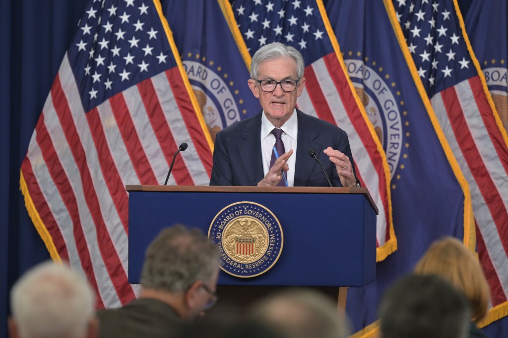
Photo of Federal Reserve Chair Jerome Powell from federalreserve.gov
Can a president fire the chair of the Federal Reserve in the same way that presidents have been able to fire cabinet secretaries? President Donald Trump has had a contentious relationship with Fed Chair Jerome Powell. Powell’s term as Fed chair is scheduled to end in May 2026. At times, Trump has indicated that he would like to remove Powell before Powell’s term ends, although most recently he’s indicated that he won’t do so.
Does Trump, or any president, have the legal authority to replace a Fed chair before the chair’s term expires? As we discuss in Macroeconomics, Chapter 27 (Economics Chapter 17), according to the Federal Reserve Act, once a Fed chair is nominated to a four-year term by the president (President Trump first nominated Powell to be chair in 2017 and Powell took office in 2018) and confirmed by the Senate, the president cannot remove the Fed chair except “for cause.” As we’ve noted in previous blog posts, most legal scholars argue that a president cannot remove a Fed chair due to a disagreement over monetary policy.
But if the Fed is part of the executive branch of the federal government and the president is the head of executive branch, why shouldn’t the president be able to replace a Fed chair. Article I, Section II of the Constitution of the United States states that: “The executive Power shall be vested in a President of the United States of America.” The ability of Congress to limit the president’s power to appoint and remove heads of commissions, agencies, and other bodies in the executive branch of government—such as the Federal Reserve—is not clearly specified in the Constitution. In 1935, a unanimous Supreme Court ruled in the case of Humphrey’s Executor v. United States that President Franklin Roosevelt couldn’t remove a member of the Federal Trade Commission (FTC) because in creating the FTC, Congress specified that members could only be removed for cause. Legal scholars have presumed that the ruling in this case would also bar attempts by a president to remove members of the Fed’s Board of Governors because of a disagreement over monetary policy.
Earlier this year, the Trump administration fired a member of the National Labor Relations Board (NLRB) and a member of the Merit Systems Protection Board (MSPB). The members sued and an appeals court ordered the president to reinstate the members. The Trump administration appealed the order to the Supreme Court, which on Thursday (May 22) granted a stay of the order on the grounds that “the Government is likely to show that both the NLRB and MSPB exercise considerable executive power,” and therefore can be removed by the president, when the case is heard by the lower court. The ruling indicated that a majority of the Supreme Court is likely to overturn the Humphrey’s Executor precedent either in this case, if it ends up being argued before the court, or in a similar case. (The Supreme Court’s order is here. An Associated Press article describing the decision is here. An article in the Wall Street Journal discussing the issues involved is here.)
Does the Supreme Court’s ruling in this case indicate that it would allow a president to remove a Fed chair? The court explicitly addressed this question, first noting that attorneys for the two board members had argued that “arguments in this case necessarily implicate the constitutionality of for-cause removal protections for members of the Federal Reserve’s Board of Governors or other members of the Federal Open Market Committee.” But the majority of the court didn’t accept the attorneys’ argument: “We disagree. The Federal Reserve is a uniquely structured, quasi-private entity that follows in the distinct historical tradition of the First and Second Banks of the United States.” (We discuss the First and Second Banks of the United States in Money, Banking, and the Financial System, Chapter 10.)
We discuss the unusual nature of the Fed’s structure in Macroeconomics, Chapter 14, Section 14.4, where we note that Congress gave the Fed a hybrid public-private structure and the ability to fund its own operations without needing appropriations from Congress. Fed Chair Powell clearly agrees that the Fed’s structure distinguishes its situation from that of other federal boards and commissions. Responding to a question following a speech in April, Powell indicated that he believes that the Fed’s unique structure means that a president would not have the power to remove a Fed chair.
It’s worth noting that the statement the court issued had the limited scope of staying the appeals court’s ruling that the members of the two commissions be reinstated. If a case arises that addresses directly the question of whether presidents can remove Fed chairs, it’s possible that, after hearing oral and written arguments, some of the justices may change their minds and decide that the president has that power. It wouldn’t be unusual for justices to change their minds during the process of deciding a case. But for now it appears that the Supreme Court would likely not allow a president to remove a Fed chair.
Since 1946, the Institute for Social Research (ISR) at the University of Michigan has conducted surveys of consumers. Each month, the ISR interviews a nationwide sample of 900 to 1,000 consumers, asking a variety of questions, including some on inflation.
The results of the University of Michigan surveys are widely reported in the business press. In the latest ISR survey it’s striking how much consumers expect inflation to increase. The median response by those surveyed to the question “By about what percent do you expect prices to go up/down on the average, during the next 12 months?” was 7.3 percent. If this expectation were to prove to be correct, inflation, as measured by the percentage change in the consumer price index (CPI), will have to more than double from its April value of 2.3 percent.
How accurately have consumers surveyed by the ISR predicted future inflation? The question is difficult to answer definitively because the survey question refers only to “prices” rather than to a measure of the price level, such as the consumer price index (CPI). Some people may have the CPI in mind when answering the question, but others may think of the prices of goods they buy regularly, such as groceries or gasoline. Nevertheless, it can be interesting to see how well the responses to the ISR survey match changes in the CPI, which we do in the following figure for the period from January 1978—when the survey began—to April 2024—the last month for which we have CPI data from the month one year in the future.
The blue line shows consumers’ expectations of what the inflation rate will be over the following year. The red line shows the inflation rate in a particular month calculated as the percentage change in the CPI from the same month in the previous year. So, for instance, in February 2023, consumers expected the inflation rate over the next 12 months to be 4.2 percent. The actual inflation, measured as the percentage change in the CPI between February 2023 and February 2024 was 3.2 percent.
The figure shows that consumers forecast inflation reasonably well. As a simple summary, the average inflation rate consumers expected over this whole period was 3.6 percent, while the actual inflation rate was 3.5 percent. So, for the period as a whole, the inflation rate that consumers expected was about the same as the actual inflation rate. The most persistent errors occurred during the recovery from the Great Recession of 2007–2008, particularly the five years from 2011 to 2016. During those five years, consumers expected inflation to be 2.5 percent or more, whereas actual inflation was typically below 2 percent.
Consumers also missed the magnitude of dramatic changes in the inflation rate. For instance, consumers did not predict how much the inflation would increase during the 1978 to 1980 period or during 2021 and early 2022. Similarly, consumers did not expect the decline in the price level from March to October 2009.
The two most recent expected inflation readings are 6.5 percent in April and, as noted earlier, 7.3 percent in May. In other words, the consumers surveyed are expecting inflation in April and May 2026 to be much higher than the 2 percent to 3 percent inflation rate most economists and Fed policymakers expect. For example, in March, the median forecast of inflation at the end of 2026 by the members of the Fed’s policymaking Federal Open Market Committee (FOMC) was only 2.2 percent. (Note, though, that FOMC members are projecting the percentage change in the personal consumption expenditures (PCE) price index rather than the percentage change in the CPI. CPI inflation has typically been higher than PCE inflation. For instance, in the period since January 1978, average CPI inflation was 3.6 percent, while average PCE inflation was 3.1 percent).
If economists and policymakers are accurately projecting inflation in 2026, it would be an unusual case of consumers in the ISR survey substantially overpredicting the rate of inflation. One possibility is that news reports of the effect of the Trump Administration’s tariff policies on the inflation rate may have caused consumers to sharply increase the inflation rate they expect next year. If, as seems likely, the tariff increases end up being much smaller than those announced on April 2, the inflation rate in 2026 may be lower than the consumers surveyed expect.
Image generated by ChatGTP-4o of a family shopping in a supermarket.
Today (May 13), the Bureau of Labor Statistics (BLS) released its report on the consumer price index (CPI) for April. The following figure compares headline inflation (the blue line) and core inflation (the green line).
The headline inflation rate, which is measured by the percentage change in the CPI from the same month in the previous year, was 2.3 percent in April—down from 2.4 percent in March.
The core inflation rate,which excludes the prices of food and energy, was 2.8 percent in April—unchanged from March.
Headline inflation was the lowest since February in 2021—before the acceleration in inflation that began in the spring of 2021. Core inflation was the lowest since March 2021. Both headline inflation and core inflation were what economists surveyed had expected.
In the following figure, we look at the 1-month inflation rate for headline and core inflation—that is the annual inflation rate calculated by compounding the current month’s rate over an entire year. Calculated as the 1-month inflation rate, headline inflation (the blue line) rose from –0.6 percent in March to 2.7 percent in April. Core inflation (the red line) rose from 0.9 percent in March to 2.9 percent in April.
The 1-month and 12-month inflation rates are telling different stories, with 12-month inflation indicating that the rate of price increase is back to what it was in early 2021. The 1-month inflation rate indicates a significant increase in April from the very low rate of price increase in March. The 1-month inflation rate indicates that inflation is still running ahead of the Fed’s 2 percent annual inflation target.
Of course, it’s important not to overinterpret the data from a single month. The figure shows that 1-month inflation is particularly volatile. It is possible, though, that the increase in 1-month inflation in April reflects the effect on the price level of the large tariff increases the Trump Administration announced on April 2. Whether those effects will persist is unclear because the administration has been engaged in negotiations that may significantly reduce the tariff increases announced in April. Finally, note that the Fed uses the personal consumption expenditures (PCE) price index, rather than the CPI, to evaluate whether it is hitting its 2 percent annual inflation target.
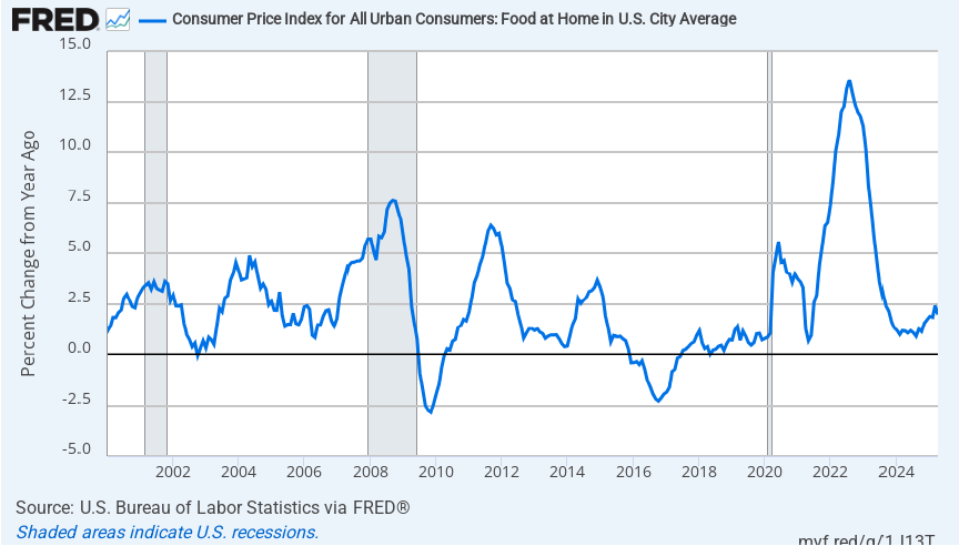
There’s been considerable discussion in the media about continuing inflation in grocery prices. The following figure shows inflation in the CPI category “food at home,” which is primarily grocery prices. Inflation in grocery prices was 2.0 percent in April and has been below 2.5 percent every month since September 2023. Over the past year, there has been a slight upward trend in inflation in grocery prices but to this point it remains relatively low, although well above the very low rates of inflation in grocery prices that prevailed from 2015 to 2019.
It’s the nature of the CPI that in any given month some prices will increase rapidly while other prices will increase slowly or even decline. Although, on average, grocery price inflation has been relatively low, there have been substantial increases in the prices of some food items. For instance, a recent article in the Wall Street Journal noted that rising cattle prices will likely be reflected in coming months rising prices for beef purchased in supermarkets. The following figure shows inflation in the prices of ground beef and steaks over the period starting in January 2015. As we should expect, the prices of these two goods are more volatile mont to month than are grocery prices as a whole. Ground beef prices increased 10.8 percent in April, an increase that will likely be noticeable to someone planning for a Memorial Day cookout.
To better estimate the underlying trend in inflation, some economists look at median inflation and trimmed mean inflation.
Median inflation is calculated by economists at the Federal Reserve Bank of Cleveland and Ohio State University. If we listed the inflation rate in each individual good or service in the CPI, median inflation is the inflation rate of the good or service that is in the middle of the list—that is, the inflation rate in the price of the good or service that has an equal number of higher and lower inflation rates.
Trimmed-mean inflation drops the 8 percent of goods and services with the highest inflation rates and the 8 percent of goods and services with the lowest inflation rates.
The following figure shows that 12-month trimmed-mean inflation (the blue line) was 3.0 percent in April, unchanged from March. Twelve-month median inflation (the red line) 3.5 percent in April, also unchanged from March.
The following figure shows 1-month trimmed-mean and median inflation. One-month trimmed-mean inflation increased from 2.6 percent in March to 3.0. percent in April. One-month median inflation declined from 4.2 percent in March to 4.0 percent in April. These data, although mixed, provide some confirmation that inflation likely increased somewhat from March to April.
What are the implications of this CPI report for the actions the FOMC may take at its next several meetings? Investors who buy and sell federal funds futures contracts still do not expect that the FOMC will cut its target for the federal funds rate at its next two meetings. (We discuss the futures market for federal funds in this blog post.) Today, investors assigned only an 8.4 percent probability to the Fed’s policymaking Federal Open Market Committee (FOMC) cutting its target from the current 4.25 percent to 4.50 percent range at its meeting on June 17–18. Investors assigned a probability of 34.9 percent that the FOMC will cut its target after its meeting on July 29–30. Investors assigned a probability of 73.1 percent that the committee will cut its target after its meeting on September 16–17. The FOMC’s actions will likely depend in part on the success of the current trade negotiations.
The economy and financial markets nervously await the July 8 end of the 90-day pause of the Trump administration’s “reciprocal” tariffs. But four days earlier, Republicans can allay those fears with a pro-growth policy that advances President Trump’s Made in America agenda without tariffs. The fix: tax reform.
July 4 is the date that Treasury Secretary Bessent has predicted Congress and the White House will have ready a 2.0 version of the landmark Tax Cut and Jobs Act of 2017, or TCJA. Without congressional action, some of these reforms will expire at the end of 2025, killing changes that still benefit the economy. Corporate tax changes, in particular, boosted investment and growth. These should remain the focal point of this next tax bill—for many reasons. Done right, corporate tax reform could advance President Trump’s goal to bring investment to American production without using economy-roiling tariffs. Call it TCJA+.
Renewing some parts of the original TCJA will help investment in the U.S. The 2017 reform offered incentives for investment in new businesses by allowing them to expense the cost of assets, rather than writing them off over time. But these benefits were set to be phased out from 2023 to 2026, removing a key pro-growth element of the earlier law.
Then there are two new provisions Republicans should add to secure Mr. Trump’s goal to have more made in America. Both were in the original 2016 House Republican tax reform blueprint.
First, Congress should change business taxation from the current income tax to a cash-flow tax, which taxes a firm’s revenue, minus all its expenses, including investment. Long championed by economists and tax-law experts, a cash-flow tax would allow businesses to expense investment immediately. It would also disallow nonfinancial companies from making interest deductions, because unlike an income tax, a cash-flow tax treats debt and equity the same. This removes an important tax incentive for firms to allow themselves to be leveraged. A cash-flow tax is also much simpler than a corporate income tax, which requires complex depreciation schedules. Most important, the reform would stimulate business investment.
Second, legislators should add a border adjustment to corporate taxes. That would deny companies a tax deduction for expenses of inputs imported from abroad, while exempting U.S. exports from taxation. As the Trump administration has observed, other countries already use border adjustments in their value-added taxes on consumption. America uses a similar mechanism in state and local retail taxes, too. If you buy a kitchen appliance in New York, you pay New York sales tax, even if it was made in Ohio. Sales tax applies only where the good is sold, not where it originates.
Though distinct from tariffs, border adjustments can promote domestic production. Adding a border adjustment to the federal corporate tax would eliminate any extra tax businesses suffer now simply as a consequence of producing in the U.S. Though the 2017 law made the U.S. tax system more globally competitive by lowering the corporate income tax rate from 35% to 21%, it’s still higher than in many other countries, which attract production with low cost. A border adjustment would remove this incentive for American firms to locate profits or activities abroad, while increasing incentives for non-U.S. firms to locate activities within our borders.
As with the original pro-investment features in the 2017 law, this TCJA+ reform would increase investment and incomes—and thereby revenue. For the original TCJA, when the Congressional Budget Office included the macroeconomic effects of higher incomes buoyed by the reforms’ pro-growth elements, the CBO reduced the estimated revenue loss from the tax cuts by almost 30%. Changing the corporate income tax to a cash-flow levy would similarly increase revenue by removing taxes on what economists call the “normal return” on investment, or the cost of capital. Companies would instead pay only on profits above this amount. A border adjustment can likewise raise substantial revenue over the next decade because imports (which would receive no deduction) are larger than exports (which would no longer be taxed).
The higher revenue these two TCJA+ provisions promise could be used to lower the tax rate on business cash flow or to fund other tax-policy objectives. Importantly, that revenue can replace revenue raised from the tariffs the Trump administration had planned to implement on July 8. These two tax provisions would accomplish the president’s America-first and revenue objectives without destabilizing businesses with whipsawing tariffs.
Finally, TCJA+ would offer another big benefit: It would move the U.S. toward independence from political meddling in the economy via targeted protection or subsidies. This added predictability and breathing room for investment would be one more reason to produce in America. Pluses indeed.
Fed Chair Jerome Powell speaking at a press conference following a meeting of the FOMC (photo from federalreserve.gov)
Members of the Fed’s policymaking Federal Open Market Committee (FOMC) had signaled clearly before today’s (May 7) meeting that the committee would leave its target range for the federal funds rate unchanged at 4.25 percent to 4.50 percent. In the statement released after its meeting, the committee made one significant change to the wording in its statement following its last meeting on March 19. The committee added the words in bold to the following sentence:
“The Committee is attentive to the risks to both sides of its dual mandate and judges that the risks of higher unemployment and higher inflation have risen.”
The key event since the last FOMC meeting was President Trump’s announcement on April 2 that he would implement tariff increases that were much higher than had previously been expected.
As we noted in an earlier blog post, an unexpected increase in tariff rates will result in an aggregate supply shock to the economy. As we discuss in Macroeconomics, Chapter 13,Section 13.3 (Economics, Chapter 23, Section 23.3), an aggregate supply shock puts upward pressure on the price level at the same time as it causes a decline in real GDP and employment. The result, as the FOMC statement indicates, can be both rising inflation and rising unemployment. If higher inflation and higher unemployment persist, the U.S. economy would be experiencing stagflation. The United States last experienced stagflation during the 1970s when large increases in oil prices caused an aggregate supply shock.
During his press conference following the meeting, Fed Chair Jerome Powell indicated that the increase in tariffs might the Fed’s dual mandate goals of price stability and maximum employment “in tension” if both inflation and unemployment increase. If the FOMC were to increase its target for the federal funds rate in order to slow the growth of demand and bring down the inflation rate, the result might be to further increase unemployment. But if the FOMC were to cut its target for the federal funds rate to increase the growth of demand and reduce the unemployment rate, the result might be to further increase the inflation rate.
Powell emphasized during his press conference that tariffs had not yet had an effect on either inflation or unemployment that was large enough to be reflected in macroeconomic data—as we’ve noted in blog posts discussing recent macroeconomic data releases. As a result, the consensus among committee members is that it would be better to wait to future meetings before deciding what changes in the federal funds rate might be needed: “We’re in a good position to wait and see. We don’t have to be in a hurry.”
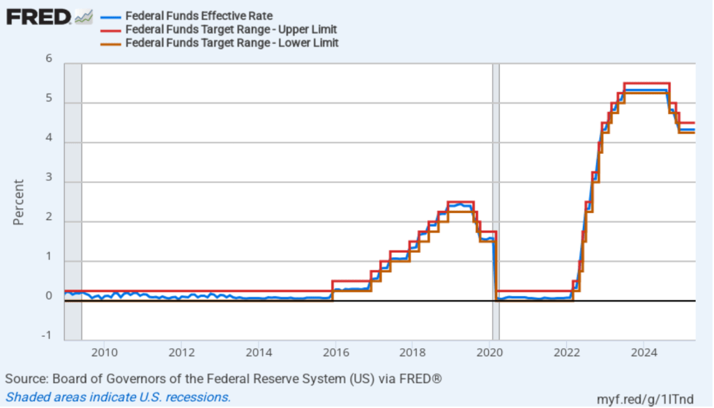
The following figure shows, for the period since January 2010, the upper bound (the blue line) and lower bound (the green line) for the FOMC’s target range for the federal funds rate and the actual values of the federal funds rate (the red line) during that time. Note that the Fed is successful in keeping the value of the federal funds rate in its target range. (We discuss the monetary policy tools the FOMC uses to maintain the federal funds rate in its target range in Macroeconomics, Chapter 15, Section 15.2 (Economics, Chapter 25, Section 25.2).)
In his press conference, Powell indicated that when the committee would change its target for the federal funds rate was dependent on the trends in macroeconomic data on inflation, unemployment, and output during the coming months. He noted that if both unemployment and inflation significantly increased, the committee would focus on which variable had moved furthest from the Fed’s target. He also noted that it was possible that neither inflation nor unemployment might end up significantly increasing either because tariff negotiations lead to lower tariff rates or because the economy proves to be better able to deal with the effects of tariff increases than many economist now expect.
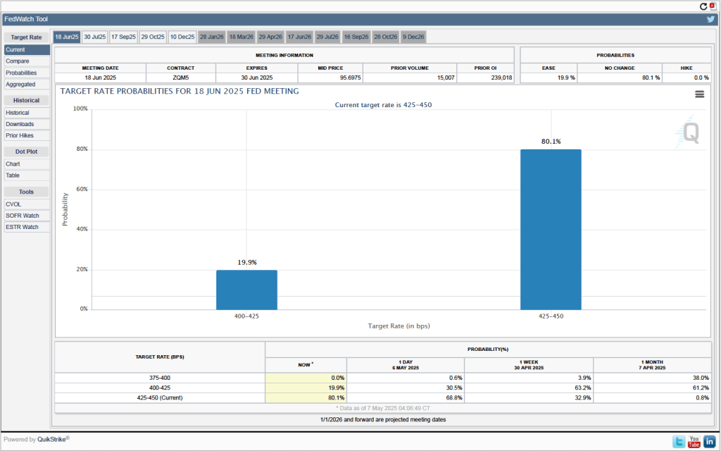
One indication of expectations of future changes in the target for the federal funds rate comes from investors who buy and sell federal funds futures contracts. (We discuss the futures market for federal funds in this blog post.) The data from the futures market indicate that investors don’t expect that the FOMC will cut its target for the federal funds rate at its May 17–18 meeting. As shown in the following figure, investors assign a 80.1 percent probability to the committee keeping its target unchanged at 4.25 percent to 4.50 percent at that meeting.
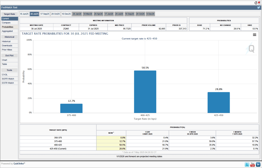
When will the Fed likely cut its target for the federal funds rate? As the following figure shows, investors expect it to happen at the FOMC’s July 29–30 meeting. Investors assign a probably of 58.5 percent to the committee cutting its target by 0.25 percentage point (25 basis points) at that meeting and a probability of 12.7 percent to the committee cutting its target by 50 basis points. Investors assign a probability of only 28.8 percent to the committee leaving its target unchanged.
Image created by ChatGTP=4o of workers on an automobile assembly line.
We noted in a blog post earlier this week that although the preliminary estimate from the Bureau of Economic Analysis (BEA) indicated that real GDP had declined during the first quarter of 2025, the report didn’t provide a clear indication that the U.S. economy was in recession. This morning (May 2), the Bureau of Labor Statistics (BLS) released its “Employment Situation” report (often called the “jobs report”) for April. The data in the report also show no sign that the U.S. economy is in a recession. Although there have been many stories in the media about businesspeople becoming increasingly pessimistic, we don’t yet see it in the employment data. We should add two caveats, however: 1. The effects of the large tariff increases the Trump Administration announced on April 2 are likely not reflected in the data from this report, and 2. at the beginning of a recession the data in the jobs report can be subject to large revisions.
The jobs report has two estimates of the change in employment during the month: one estimate from the establishment survey, often referred to as the payroll survey, and one from the household survey. As we discuss in Macroeconomics, Chapter 9, Section 9.1 (Economics, Chapter 19, Section 19.1), many economists and Federal Reserve policymakers believe that employment data from the establishment survey provide a more accurate indicator of the state of the labor market than do the household survey’s employment data and unemployment data. (The groups included in the employment estimates from the two surveys are somewhat different, as we discuss in this post.)
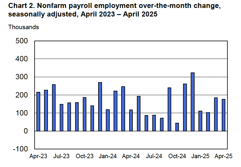
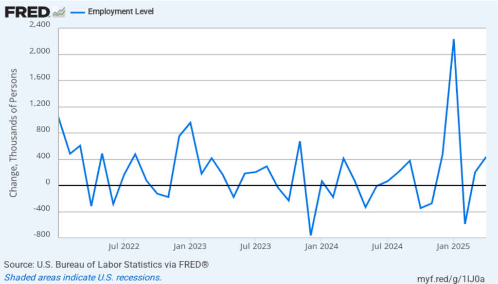
According to the establishment survey, there was a net increase of 177,000 jobs during April. This increase was well above the increase of 135,000 that economists surveyed had forecast. Somewhat offsetting this unexpectedly large increase was the BLS revising downward its previous estimates of employment in February and March by a combined 58,000 jobs. (The BLS notes that: “Monthly revisions result from additional reports received from businesses and government agencies since the last published estimates and from the recalculation of seasonal factors.”) The following figure from the jobs report shows the net change in payroll employment for each month in the last two years.
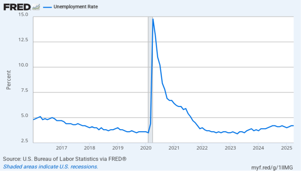
The unemployment rate was unchanged to 4.2 percent in April. As the following figure shows, the unemployment rate has been remarkably stable over the past year, staying between 4.0 percent and 4.2 percent in each month since May 2024. In March, the members of the Federal Open Market Committee (FOMC) forecast that the unemployment rate for 2025 would average 4.4 percent.
As the following figure shows, the monthly net change in jobs from the household survey moves much more erratically than does the net change in jobs from the establishment survey. As measured by the household survey, there was a net increase of 436,000 jobs in April, following an increase of 201,000 jobs in March. As an indication of the volatility in the employment changes in the household survey note the very large swings in net new jobs in January and February. In any particular month, the story told by the two surveys can be inconsistent with employment increasing in one survey while falling in the other. This month, however, both surveys showed net jobs increasing. (In this blog post, we discuss the differences between the employment estimates in the two surveys.)
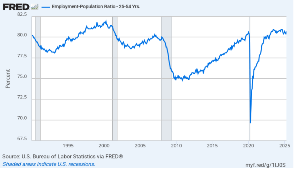
The household survey has another indication of continuing strength in the labor market. The employment-population ratio for prime age workers—those aged 25 to 54—increased from 80.4 percent in March to 80.7 percent in April. The prime-age employment-population ratio is somewhat below the high of 80.9 percent in mid-2024, but is above what the ratio was in any month during the period from January 2008 to January 2020.
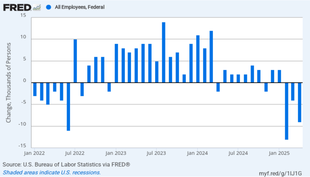
It remains unclear how many federal workers have been laid off since the Trump Administration took office. The establishment survey shows a decline in total federal government employment of 9,000 in April. However, the BLS notes that: “Employees on paid leave or receiving ongoing severance pay are counted as employed in the establishment survey.” It’s possible that as more federal employees end their period of receiving severance pay, future jobs reports may find a more significant decline in federal employment. To this point, the decline in federal employment has been too small to have a significant effect on the overall labor market.
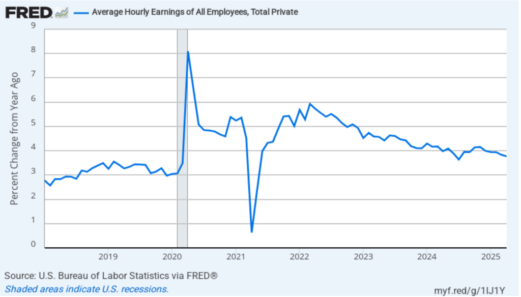
The establishment survey also includes data on average hourly earnings (AHE). As we noted in this post, many economists and policymakers believe the employment cost index (ECI) is a better measure of wage pressures in the economy than is the AHE. The AHE does have the important advantage of being available monthly, whereas the ECI is only available quarterly. The following figure shows the percentage change in the AHE from the same month in the previous year. The AHE increased 3.8 percent in April, which is unchanged from the March increase.
The following figure shows wage inflation calculated by compounding the current month’s rate over an entire year. (The figure above shows what is sometimes called 12-month wage inflation, whereas this figure shows 1-month wage inflation.) One-month wage inflation is much more volatile than 12-month wage inflation—note the very large swings in 1-month wage inflation in April and May 2020 during the business closures caused by the Covid pandemic. The April, the 1-month rate of wage inflation was 2.0 percent, down from 3.4 percent in March. If the 1-month increase in AHE is sustained, it would contribute to the Fed’s achieving its 2 percent target rate of price inflation.
Today’s jobs report leaves the situation facing the Federal Reserve’s policy-making Federal Open Market Committee (FOMC) largely unchanged. Looming over monetary policy, however, is the expected effect of the Trump Administration’s unexpectedly large tariff increases. As we note in this blog post, a large unexpected increase in tariffs results in an aggregate supply shock to the economy. In terms of the basic aggregate demand and aggregate supply model that we discuss in Macroeconomics, Chapter 13 (Economics, Chapter 23), an unexpected increase in tariffs shifts the short-run aggregate supply curve (SRAS) to the left, increasing the price level and reducing the level of real GDP.
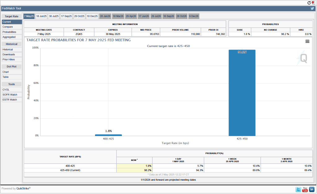
One indication of expectations of future changes in the target for the federal funds rate comes from investors who buy and sell federal funds futures contracts. (We discuss the futures market for federal funds in this blog post.) The data from the futures market indicate that, despite the potential effects of the surprisingly large tariff increases, investors don’t expect that the FOMC will cut its target for the federal funds rate at its May 6–7 meeting. As shown in the following figure, investors assign a 98.2 percent probability to the committee keeping its target unchanged at 4.25 percent to 4.50 percent at that meeting.
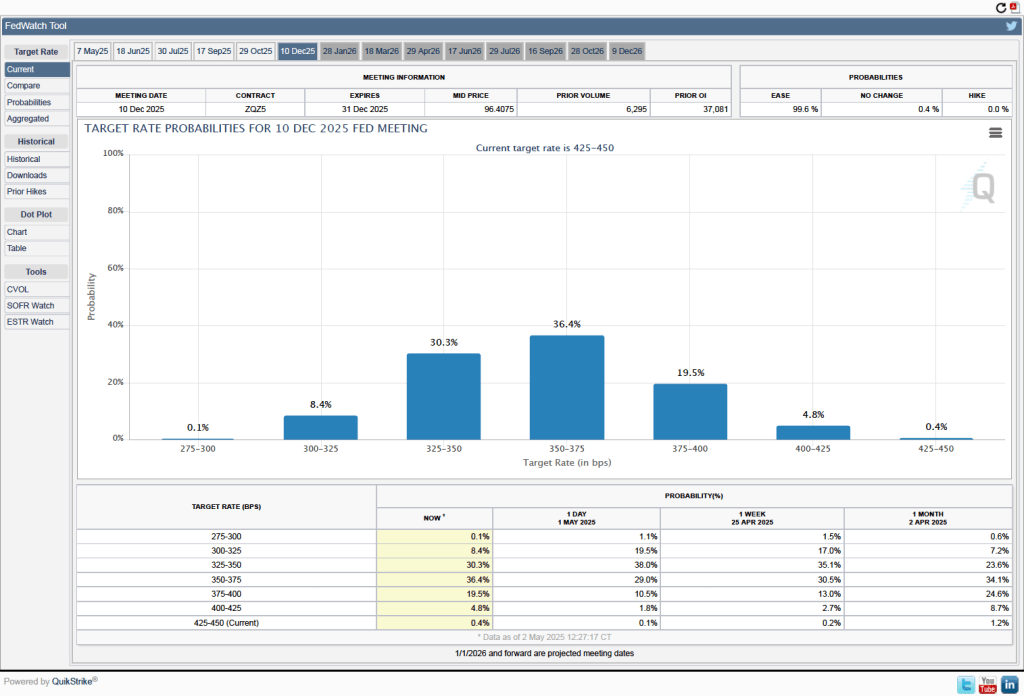
It’s a different story if we look at the end of the year. As the following figure shows, investors now expect that by the end of the FOMC’s meeting on December 9-10, the committee will have implemented at least three 0.25 percentage point (25 basis points) cuts in its target range for the federal funds rate. Investors assign a probability of 75.9 percent that the target range will end the year at 3.50 percent to 3.75 percent or lower. At their March meeting, FOMC members projected only two 25 basis point cuts this year—but that was before the announcement of the unexpectedly large tariff increases.
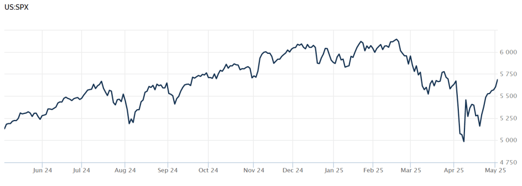
How the economy will fare for the remainder of the year depends heavily on what happens with respect to tariffs. News today that China and the United States may be negotiating lower tariff rates has contributed to rising stock prices. The following figure from the Wall Street Journal shows movements in the S&P stock index over the past year. The index declined sharply on April 2, following President Trump’s announcement of the tariff increases. As of 2 pm today, the S&P index has risen above its value on April 1, meaning that it has recovered all of the losses since the announcement of the tariff increases. The increase in stock prices likely indicates that investors expect that the tariff increases will end up being much smaller than those originally announced and that the chances of a recession happening soon are lower than they appeared to be on April 2.
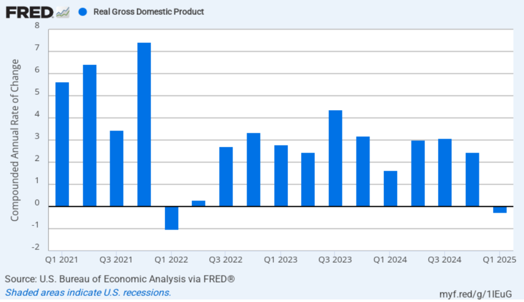
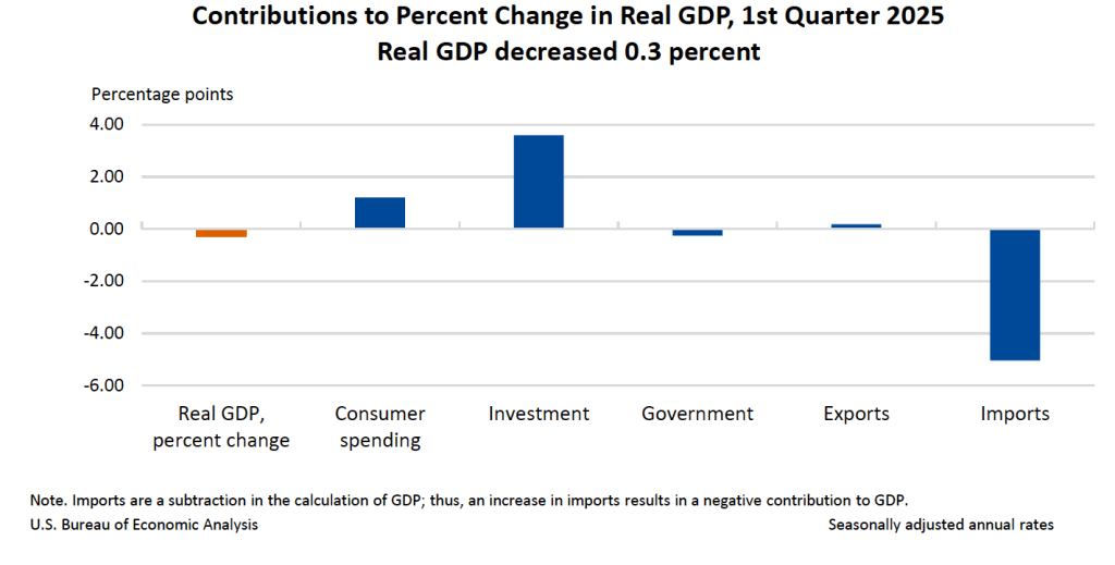
This morning (April 30), the Bureau of Economic Analysis (BEA) released its advance estimate of GDP for the first quarter of 2025. (The report can be found here.) The BEA estimates that real GDP fell by 0.3 percent, measured at an annual rate, in the first quarter—January through March. Economists surveyed had expected an 0.8 percent increase. Real GDP grew by an estimated 2.5 percent in the fourth quarter of 2024. The following figure shows the estimated rates of GDP growth in each quarter beginning in 2021.
As the following figure—taken from the BEA report—shows, the increase in imports was the most important factor contributing to the decline in real GDP. The quarter ended before the Trump Administration announced large tariff increases on April 2, but the increase in imports is likely attributable to firms attempting to beat the tariff increases they expected were coming.
It’s notable that the change in real private inventories was a large $140 billion, which contributed 2.3 percentage points to the change in real GDP. Again, it’s likely that the large increase in inventories represented firms stockpiling goods in anticipation of the tariff increases.
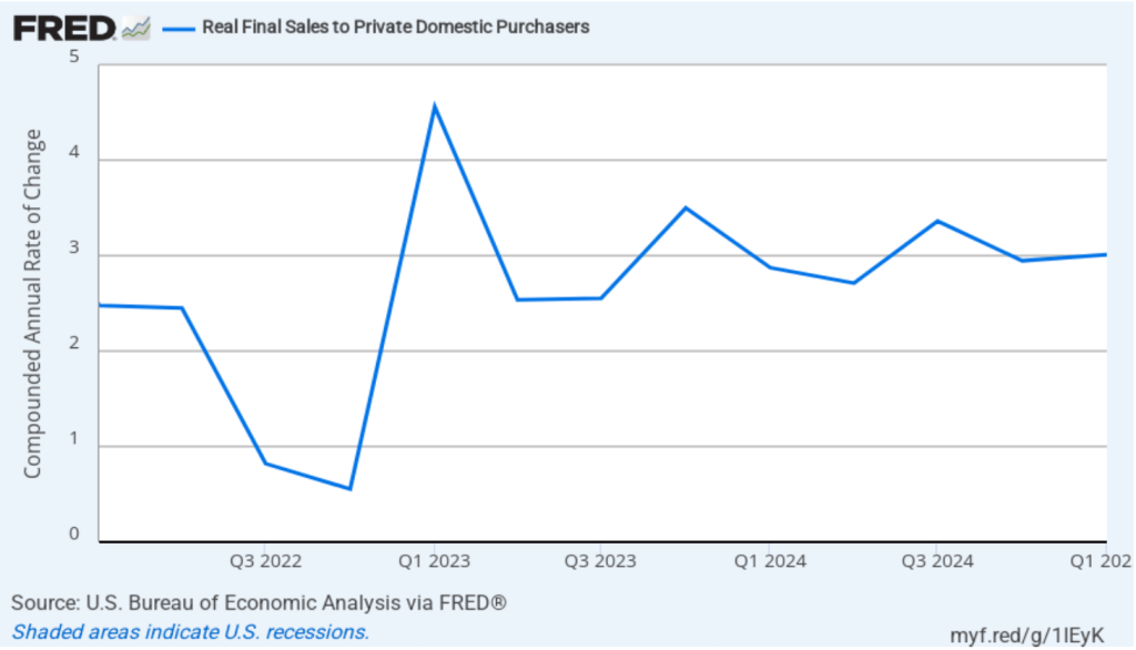
One way to strip out the effects of imports, inventory investment, and government purchases—which can also be volatile—is to look at real final sales to domestic purchasers, which includes only spending by U.S. households and firms on domestic production. As the following figure shows, real final sales to domestic purchasers increase by 3.0 percent in the first quarter of 2024, which was a slight increase from the 2.9 percent increase in the fourth quarter of 2024. The large difference between the change in real GDP and the change in real final sales to domestic purchasers is an indication of how strongly this quarter’s national income data were affected by businesses anticipating the tariff increases.
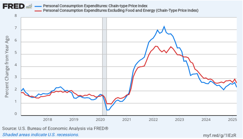
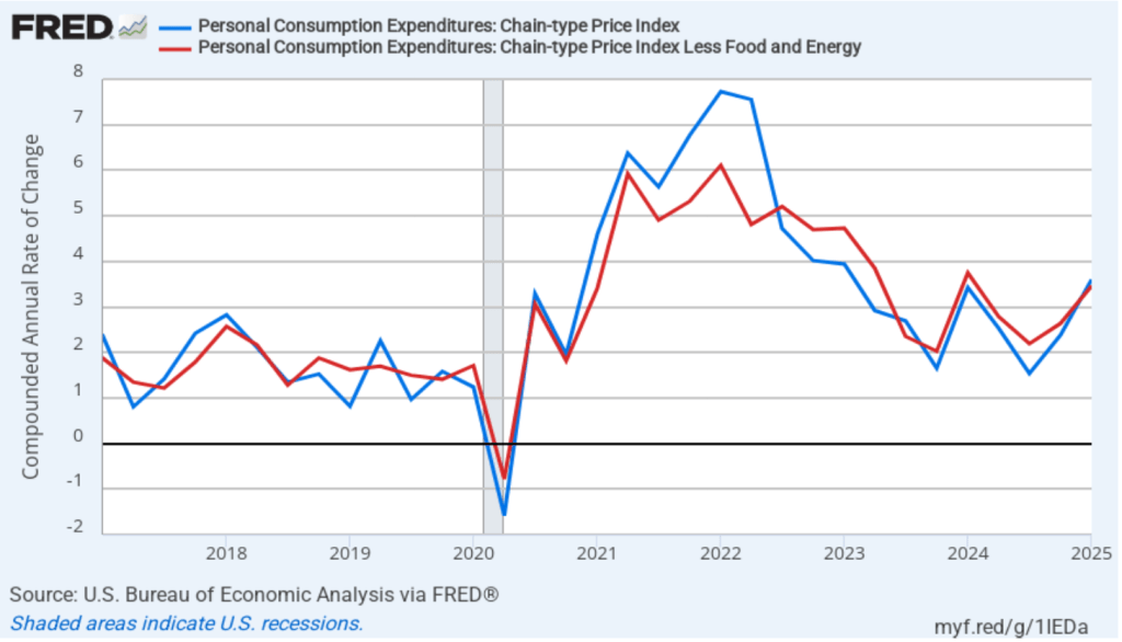
In the separate “Personal Income and Outlays” report that the BEA also released this morning, the bureau reported monthly data on the personal consumption expenditures (PCE) price index. The Fed relies on annual changes in the PCE price index to evaluate whether it’s meeting its 2 percent annual inflation target. The following figure shows PCE inflation (the blue line) and core PCE inflation (the red line)—which excludes energy and food prices—for the period since January 2017 with inflation measured as the percentage change in the PCE from the same month in the previous year. In March, PCE inflation was 2.3 percent, down from 2.7 percent in February. Core PCE inflation in March was 2.6 percent, down from 3.0 percent in February. Both headline and core PCE inflation were higher than the forecasts of economists surveyed.
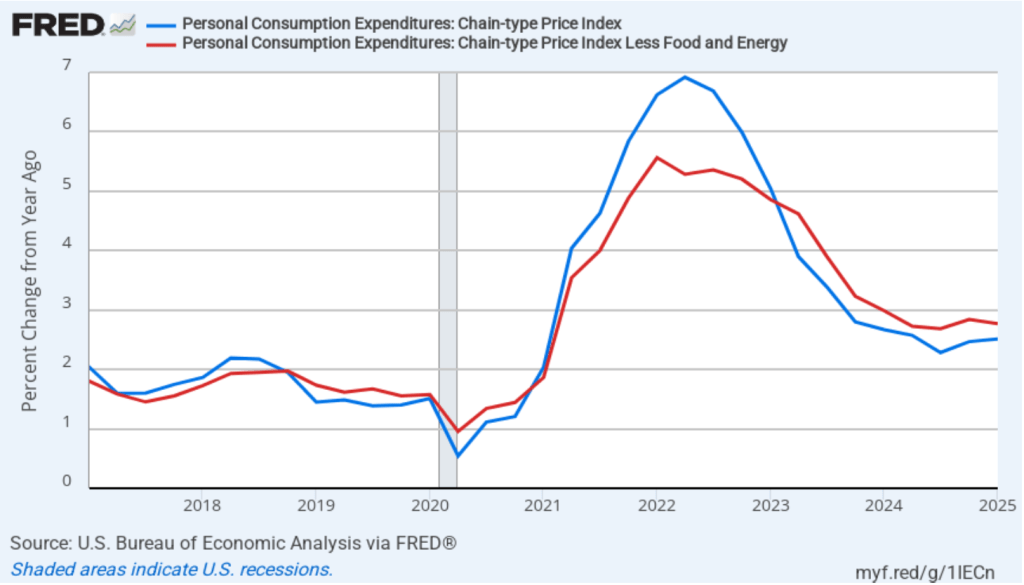
The BEA also released quarterly PCE data as part of its GDP report. The following figure shows quarterly headline PCE inflation (the blue line) and core PCE inflation (the red line). Inflation is calculated as the percentage change from the same quarter in the previous year. Headline PCE inflation in the first quarter was 2.5 percent, unchanged from the fourth quarter of 2025. Core PCE inflation was 2.8 percent, also unchanged from the fourth quarter of 2025. Both measures were still above the Fed’s 2 percent inflation target.
The following figure shows quarterly PCE inflation and quarterly core PCE inflation calculated by compounding the current quarter’s rate over an entire year. Measured this way, headline PCE inflation increased from 2.4 percent in the fourth quarter of 2024 to 3.6 percent in the first quarter of 2025. Core PCE inflation increased from 2.6 percent in the fourth quarter of 2024 to 3.5 percent in the first quarter of 2025. Clearly, the quarterly data show significantly higher inflation than do the monthly data. As we discuss in this blog post, tariff increases result in an aggregate supply shock to the economy. As a result, unless the current and scheduled tariff increases are reversed, we will likely see a significant increase in inflation in the coming months. So, neither the monthly nor the quarterly PCE data may be giving a good indication of the course of future inflation.
What should we make of today’s macro data releases? First, it’s important to remember that these data will be subject to revisions in coming months. If we are heading into a recession, the revisions may well be very large. Second, we are sailing into unknown waters because the U.S. economy hasn’t experienced tariff increases as large as these since passage of the Smoot-Hawley Tariff in 1930. Third, at this point we don’t know whether some, most, all, or none of the tariff increases will be reversed as a result of negotiations during the coming weeks. Finally, on Friday, the Bureau of Labor Statistics will release its “Employment Situation Report” for March. That report will provide some additional insight into the state of the economy—as least as it was in March before the full effects of the tariffs have been felt.
An image generated by ChatGTP-4o of a hypothetical meeting between President Richard Nixon and Fed Chair Arthur Burns in the White House.
In a speech on April 15 at the Economic Club of Chicago, Federal Reserve Chair Jerome Powell discussed how the Fed might react to President Donald Trump’s tariff increases: “Tariffs are highly likely to generate at least a temporary rise in inflation. The inflationary effects could also be more persistent…. Our obligation is to keep longer-term inflation expectations well anchored and to make certain that a one-time increase in the price level does not become an ongoing inflation problem.”
Powell’s remarks were interpreted as indicating that the Fed’s policymaking Federal Open Market Committee (FOMC) was unlikely to cut its target for the federal funds rate anytime soon. President Trump, who has stated several times that the FOMC should cut its target, was displeased with Powell’s position and posted on social media that “Powell’s termination cannot come fast enough!” Stock prices declined sharply on the possibility that Trump might try to fire Powell because many economists and market participants believed that move would increase uncertainty and possibly undermine the FOMC’s continuing attempts to bring inflation down to the Fed’s 2 percent target. Trump, possibly responding to the fall in stock prices, stated to reporters that he had “no intention” of firing Powell. In this recent blog post we discuss the debate over whether presidents can legally fire Fed chairs.
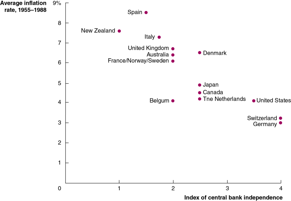
Leaving aside the legal issue of whether a president can fire a Fed chair, would it be better or worse for the conduct of monetary if the presdient did have that power? We review the arguments for and against the Fed conducting monetary policy independently of the president and Congress in Macroeconomics, Chapter 17, Section 17.4 (Economics, Chapter 27, Section 27.4). One key point that’s often made in favor of Fed independence is illustrated in Figure 17.12, which is reproduced below.
The figure is from a classic study by Alberto Alesina and Lawrence Summers, who were both economists at Harvard University at the time. Alesina and Summers tested the assertion that the less independent a country’s central bank, the higher the country’s inflation rate will be by comparing the degree of central bank independence and the inflation rate for 16 high-income countries during the years from 1955 to 1988. As the figure shows, countries with highly independent central banks, such as the United States, Switzerland, and Germany, had lower inflation rates than countries whose central banks had little independence, such as New Zealand, Italy, and Spain. In the following years, New Zealand and Canada granted their banks more independence, at least partly to better fight inflation.
Debates over Fed independence didn’t start with President Trump and Fed Chair Powell; they date all the way back to the passage of the Federal Reserve Act in 1913. The background to the passage of the Act is the political struggle over establishing a central bank during the early years of the country. In 1791, Congress established the Bank of the United States, at the urging of the country’s first Treasury secretary, Alexander Hamilton. When the bank’s initial 20-year charter expired in 1811, political opposition kept the charter from being renewed, and the bank went out of existence. The bank’s opponents believed that the bank’s actions had the effect of reducing loans to farmers and owners of small businesses and that Congress had exceeded its constitutional authority in establishing the bank. Financial problems during the War of 1812 led Congress to charter the Second Bank of the United States in 1816. But, again, political opposition, this time led by President Andrew Jackson, resulted in the bank’s charter not being renewed in 1836.
As we discuss in Chapter 14, Section 14.4, Congress established the Federal Reserve as a lender of last resort to bring an end to bank panics. In 1913, Congress was less concerned aboout making the Fed independent from Congress and the president than it was in overcoming political opposition to establishing a central bank located in Washington, DC. Accordingly, Congress established a decentralized system by having 12 District Banks that would be owned by the member banks in the district. Congress gave the responsibility for overseeing the system to the Federal Reserve Board, which was the forerunner of the current Board of Governors. The president had a greater influence on the Federal Reserve Board than presidents today have on the Board of Governors because the Federal Reserve Board included the secretary of the Treasury and the comptroller of the currency as members. Then as now, the president is free to replace the secretary of the Treasury and the comptroller of the currency at any time.
When the United States entered World War I in April 1917, the Fed came under pressure to help the Treasury finance the war by making loans to banks to help the banks purchase Treasury securities—Liberty Bonds—and by lending funds to banks that banks could loan to households to purchase bonds. In 1919, a ruling by the attorney general clarified that Congress had intended in the Federal Reserve Act to give the Federal Reserve Board the power to set the discounts rate the 12 District Banks charged member banks on loans.
Despite this ruling, authority within the Fed remained much more divided than is true today. Divided authority proved to be a serious problem when the Fed had to deal with the Great Depression, which began in August 1929 and worsened as the result of a series of bank panics. As we’ve seen, the secretary of the Treasury and the comptroller of the currency, both of whom report directly to the president of the United States, served on the Federal Reserve Board. So, the Fed had less independence from the executive branch of the government than it does today.
In addition, the heads of the 12 District Banks operated much more independently than they do today, with the head of the Federal Reserve Bank of New York having nearly as much influence within the system as the head of the Federal Reserve Board. At the time of the bank panics, George Harrison, the head of the Federal Reserve Bank of New York, served as chair of the Open Market Policy Conference, the predecessor of the current Federal Open Market Committee. Harrison frequently acted independently of Roy Young and Eugene Meyer, who served as heads of the Federal Reserve Board during those years. Important decisions could be made only with the consensus of these different groups. During the early 1930s, consensus proved hard to come by, and taking decisive policy actions was difficult.
The difficulties the Fed had in responding to the Great Depression led Congress to reorganize the system with the passage of the Banking Act of 1935. Most of the current structure of the Fed was put in place by that law. Power was concentrated in the hands of the Board of Governors. The removal of the secretary of the Treasury and the comptroller of the currency from the Board reduced the ability of the president to influence the Fed’s decisions.
During World War II, the Fed again came under pressure to help the federal government finance the war. The Fed agreed to hold interest rates on Treasury securities at low levels: 0.375% on Treasury bills and 2.5% on Treasury bonds. The Fed could keep interest rates at these low levels only by buying any bonds that were not purchased by private investors, thereby fixing, or pegging, the rates.
When the war ended in 1945, the Treasury and President Harry Truman wanted to continue this policy, but the Fed didn’t agree. The Fed’s concern was inflation: Larger purchases of Treasury securities by the Fed could increase the growth rate of the money supply and the rate of inflation. Fed Chair Marriner Eccles strongly objected to the policy of fixing interest rates. His opposition led President Truman to not reappoint him as chair in 1948,although Eccles continued to fight for Fed independence during the remainder of his time as a governor. On March 4, 1951, the federal government formally abandoned the wartime policy of fixing the interest rates on Treasury securities with the Treasury–Federal Reserve Accord. This agreement was important in eestablishing the Fed’s ability to operate independently of the Treasury.
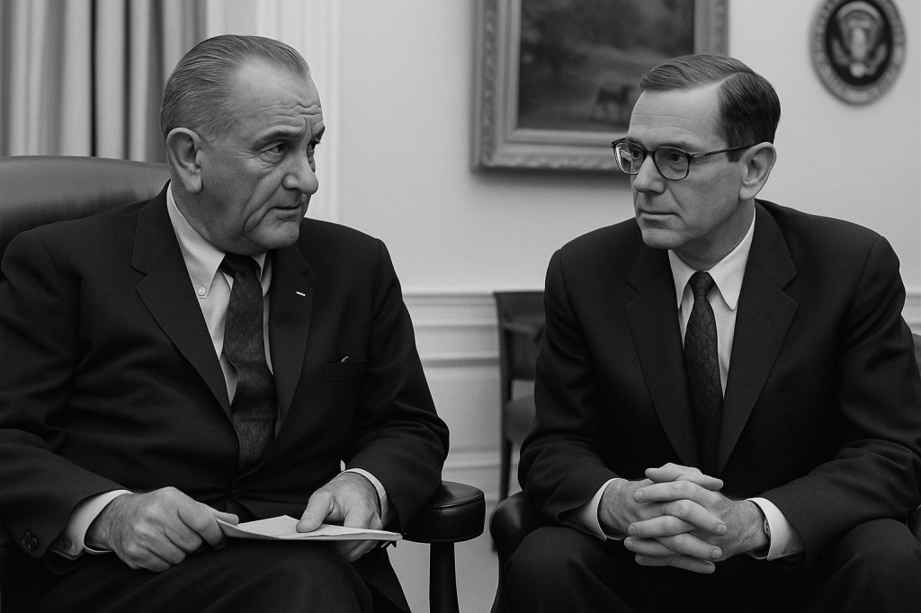
Conflicts between the Treasury and the Fed didn’t end with that agreement, however. Thomas Drechsel of the University of Maryland has analyzed the daily schedules of presidents during the period from 1933 to 2016 and finds that during these years presidents met with Fed officials on more than 800 occasions. Of course, not all of these interactions involved attempts by a president to influence the actions of a Fed Chair, but some seem to have. For example, research by Helen Fessenden of the Federal Reserve Bank of Richmond has shown that in 1967, President Lyndon Johnson, who was facing reelection in 1968, was anxious that Fed Chair William McChesney Martin adopt a more expansionary monetary policy. There is some evidence that Johnson and Martin came to an agreement that if Johnson agreed to push Congress to increase taxes, Martin would pursue an expansionary monetary policy.
An image generated by ChatGTP-4o of a hypothetical meeting between President Lyndon Johnson and Fed Chair William McChesney Martin in the White House.
Similarly, in late 1971, President Richard Nixon was concerned that the unemployment rate was at 6%, which he believed would, if it persisted, endanger his chance of reelection in 1972. Dreschel finds that Nixon met with Fed Chair Arthur Burns 34 times during the second half of 1971. Evidence from tape recordings of Nixon’s conversations with Burns at the White House and from Burns’s diary entries indicate that Nixon pressured Burns to increase the rate of growth of the money supply and that Burns agreed to do so.
President Ronald Reagan and Federal Reserve Chair Paul Volcker argued over who was at fault for the severe economic recession of the early 1980s. Reagan blamed the Fed for soaring interest rates. Volcker held that the Fed could not take action to bring down interest rates until the budget deficit—which results from policy actions of the president and Congress—was reduced. Similar conflicts occurred during the administrations of George H.W. Bush and Bill Clinton, with the Treasury frequently pushing for lower short-term interest rates than the Fed considered advisable.
During the financial crisis of 2007–2009 and during the 2020 Covid pandemic, the Fed worked closely with the Treasury. The relationship was so close, in fact, that some economists and policymakers worried that the Fed might be sacrificing some of its independence. The frequent consultations between Fed Chair Ben Bernanke and Treasury Secretary Henry Paulson in the fall of 2008, during the height of the crisis, were a break with the tradition of Fed chairs formulating policy independently of a presidential administration. During the 2020 pandemic, Fed Chair Jerome Powell and Treasury Secretary Steven Mnuchin also frequently consulted on policy.
These examples from the Fed’s history indicate that presidents have persistently attempted to influence Fed policy. Most economists believe that central bank independence is an important check on inflation. But, given the importance of monetary policy, it’s probably inevitable that presidents and members of Congress will continue to attempt to sway Fed policy.
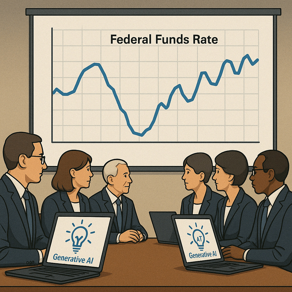
Image generated by ChatGTP-4o One of the key issues in monetary policy—dating back decades—is whether policy should be governed by a rule or whether the members of the Federal Open Market Committee (FOMC) should make “data-driven” decisions. Currently, the FOMC believes that the best approach is to let macroeconomic data drive decisions about the appropriate target … Continue reading “Should We Turn Monetary Policy over to Generative Artificial Intelligence?”
Image generated by ChatGTP-4o
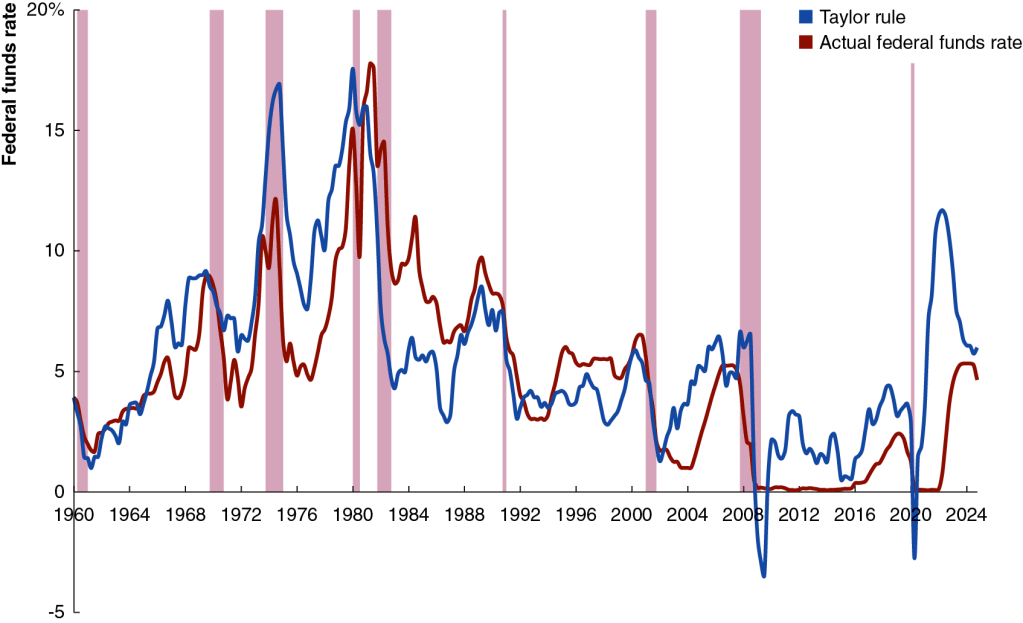
One of the key issues in monetary policy—dating back decades—is whether policy should be governed by a rule or whether the members of the Federal Open Market Committee (FOMC) should make “data-driven” decisions. Currently, the FOMC believes that the best approach is to let macroeconomic data drive decisions about the appropriate target for the federal funds rate rather than to allow a policy rule to determine the target.
In its most recent Monetary Policy Report to Congress, the Fed’s Board of Governors noted that policy rules “can provide useful benchmarks for the consideration of monetary policy. However, simple rules cannot capture all of the complex considerations that go into the formation of appropriate monetary policy, and many practical considerations make it undesirable for the FOMC to adhere strictly to the prescriptions of any specific rule.” We discuss the debate over monetary policy rules—sometimes described as the debate over “rules versus discretion” in conducting policy—in Macroeconomics, Chapter 15, Section 15.5 (Economics, Chapter 25, Section 25.5.)
Probably the best known advocate of the Fed relying on policy rules is John Taylor of Stanford University. The Taylor rule for monetary policy begins with an estimate of the value of the real federal funds rate, which is the federal funds rate—adjusted for inflation—that would be consistent with real GDP being equal to potential real GDP in the long run. With real GDP equal to potential real GDP, cyclical unemployment should be zero, and the Fed will have attained its policy goal of maximum employment, as the Fed defines it.
According to the Taylor rule, the Fed should set its current federal funds rate target equal to the sum of the current inflation rate, the equilibrium real federal funds rate, and two additional terms. The first of these terms is the inflation gap—the difference between current inflation and the target rate (currently 2 percent, as measured by the percentage change in the personal consumption expenditures (PCE) price index; the second term is the output gap—the percentage difference of real GDP from potential real GDP. The inflation gap and the output gap are each given “weights” that reflect their influence on the federal funds rate target. With weights of one-half for both gaps, we have the following Taylor rule:
Federal funds rate target = Current inflation rate + Equilibrium real federal funds rate + (1/2 × Inflation gap) + (1/2 × Output gap).
So when the inflation rate is above the Fed’s target rate, the FOMC will raise the target for the federal funds rate. Similarly, when the output gap is negative—that is, when real GDP is less than potential GDP—the FOMC will lower the target for the federal funds rate. In calibrating this rule, Taylor assumed that the equilibrium real federal funds rate is 2 percent and the target rate of inflation is 2 percent. (Note that the Taylor rule we are using here was the one Taylor first proposed in 1993. Since that time, Taylor and other economists have also analyzed other similar rules with, for instance, an assumption of a lower equilibrium real federal funds rate.)
The following figure shows the level of the federal funds rate that would have occurred if the Fed had strictly followed the original Taylor rule (the blue line) and the actual federal funds rate (the red line). The figure indicates that because during many years the two lines are close together, the Taylor rule does a reasonable job of explaining Federal Reserve policy. There are noticeable exceptions, however, such as the period of high inflation that began in the spring of 2021. During that period, the Taylor rule indicates that the FOMC should have begun raising its target for the federal funds rate earlier and raised it much higher than it did.
Taylor has presented a number of arguments in favor of the Fed relying on a rule in conducting monetary policy, including the following:
A simple policy rule (such as the Taylor rule) makes it easier for households, firms, and investors to understand Fed policy.
Conducting policy according to a rule makes it less likely that households, firms, and investors will be surprised by Fed policy.
Fed policy is less likely to be subject to political pressure if it follows a rule: “If monetary policy appears to be run in an ad hoc and complicated way rather than a systematic way, then politicians may argue that they can be just as ad hoc and interfere with monetary policy decisions.”
Following a rule makes it easier to hold the Fed accountable for policy errors.
The Fed hasn’t been persuaded by Taylor’s arguments, preferring its current data-driven approach. In setting monetary policy, the members of the FOMC believe in the importance of being forward looking, attempting to take into account the future paths of inflation and unemployment. But committee members can struggle to accurately forecast inflation and unemployment. For instance, at the time of the June 2021 meeting of the FOMC, inflation had already risen above 4%. Nevertheless, committee members forecast that inflation in 2022 would be 2.1%. Inflation in 2022 turned out to be much higher—6.6%.
To succeed with a data-driven approach to policy, members of the FOMC must be able to correctly interpret the importance of new data on economic variables as it becomes available and also accurately forecast the effects of policy changes on key variables, particularly unemployment and inflation. How do the committee members approach these tasks? To some extent they rely on formal economic models, such as those developed by the economists on the committee’s staff. But, judging by their speeches and media interviews, committee members also rely on qualitative analysis in interpreting new data and in forming their expectations of how monetary policy will affect the economy.
In recent years, generative artificial intelligence (AI) and machine learning (ML) programs have made great strides in analyzing large data sets. Should the Fed rely more heavily on these programs in conducting monetary policy? The Fed is currently only in the beginning stages of incorporating AI into its operations. In 2024, the Fed appointed a Chief Artificial Intelligence Officer (CAIO) to coordinate its AI initiatives. Initially, the Fed has used AI primarily in the areas of supervising the payment system and promoting financial stability. AI has the ability to quickly analyze millions of financial transactions to identify those that may be fraudulent or may not be in compliance with financial and banking regulations. How households, firms, and investors respond to Fed policies is an important part of how effective the policies will be. The Fed staff has used AI to analyze how financial markets are likely to react to FOMC policy announcements.
The Central Bank of Canada has gone further than the Fed in using AI. According to Tiff Macklem, the Governor of the Bank of Canada, AI is used to:
• forecast inflation, economic activity and demand for bank notes • track sentiment in key sectors of the economy • clean and verify regulatory data • improve efficiency and de-risk operations
Will central banks begin to use AI to carry out the key activity of setting policy interest rates, such as the federal funds rate in the United States? AI has the potential to adjust the federal funds rate more promptly than the members of the FOMC are able to do in their eight yearly meetings. Will it happen? At this point, generative AI and ML models are not capable of taking on that responsibility. In addition, as noted earlier, Taylor and other supporters of rules-based policies have argued that simple rules are necessary for the public to understand Fed policy. AI generated rules are likely to be too complex to be readily understood by non-specialists.
It’s too early in the process of central banks adopting AI in their operations to know the eventual outcome. But AI is likely to have a significant effect on central banks, just as it is already affecting many businesses.
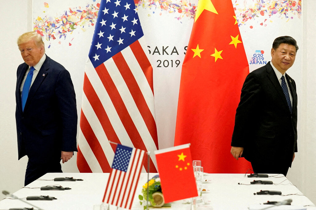
Photo of U.S. President Donald Trump and China President Xi Jinping from Reuters.
The tit-for-tat tariff increases the U.S. and Chinese governments have levied on each other’s imports have reached dizzying heights today (April 11). The United States has imposed a tariff rate of 134.7 percent on imports from China, while China has imposed a tariff rate of 147.6 percent on imports from the United States. On all other countries—the rest of the world (ROW)—the United States imposes an average tariff rate of 10.5 percent, which is a sharp increase reflecting the Trump Administration’s imposition of a tariff of at least 10 percent on all countries. The government of China imposes a tariff rate of 6.5 percent on the ROW.
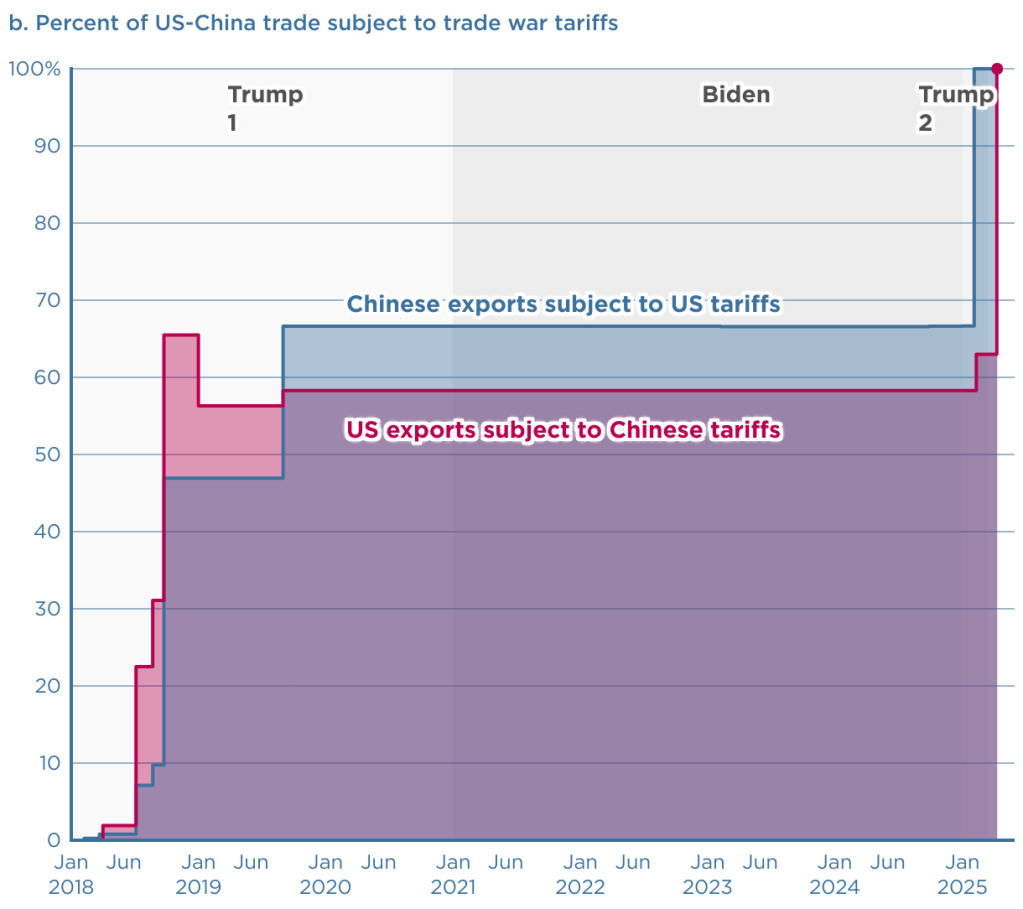
The Peterson Institute for International Economics (PIIE) is a think tank located in Washington, DC. Chad Brown, a senior fellow at PIIE, has created two charts that dramatically illustrate the current state of the U.S.-China trade war. The first chart shows the changes since the beginning of the first Trump Administration in 2017 in the tariff rates the countries have imposed on each other’s imports.
The second chart shows the percentage of each country’s exports to the other country that have been subject to tariffs. As of today, 100 percent of each country’s exports are subject to the other country’s tariffs.
Finally, we repeat a figure from an earlier blog post showing changes over time in the average tariff rate the United States levies on imports. The value for 2025 of 16.5 percent is an estimate by the Tax Foundation and assumes that the tariff rates that the Trump Administration announced on April 2 go into force, although the rates are currently suspended for 90 days—apart from those imposed on China. (An average tariff rate of 16.5 percent would be the highest levied by the United States since 1937.)
Thanks to Fernando Quijano for preparing this figure.