Photo courtesy of Lena Buonanno.
This morning of Friday, February 2, the Bureau of Labor Statistics (BLS) issued its “Employment Situation Report” for January 2024. Economists and policymakers—notably including the members of the Fed’s Federal Open Market Committee (FOMC)—typically focus on the change in total nonfarm payroll employment as recorded in the establishment, or payroll, survey. That number gives what is generally considered to be the best gauge of the current state of the labor market.
Economists surveyed in the past few days by business news outlets had expected that growth in payroll employment would slow to an increase of between 180,000 and 190,000 from the increase in December, which the BLS had an initially estimated as 216,00. (For examples of employment forecasts, see here and here.) Instead, the report indicated that net employment had increased by 353,000—nearly twice the expected amount. (The full report can be found here.)
In this previous blog post on the December employment report, we noted that although the net increase in employment in that month was still well above the increase of 70,000 to 100,000 new jobs needed to keep up with population growth, employment increases had slowed significantly in the second half of 2023 when compared with the first.
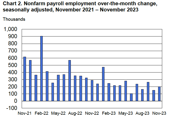
That slowing trend in employment growth did not persist in the latest monthly report. In addition, to the strong January increase of 353,000 jobs, the November 2023 estimate was revised upward from 173,000 jobs to 182,000 jobs, and the December estimate was substantially revised from 216,000 to 333,000. As the following figure from the report shows, the net increase in jobs now appears to have trended upward during the last three months of 2023.

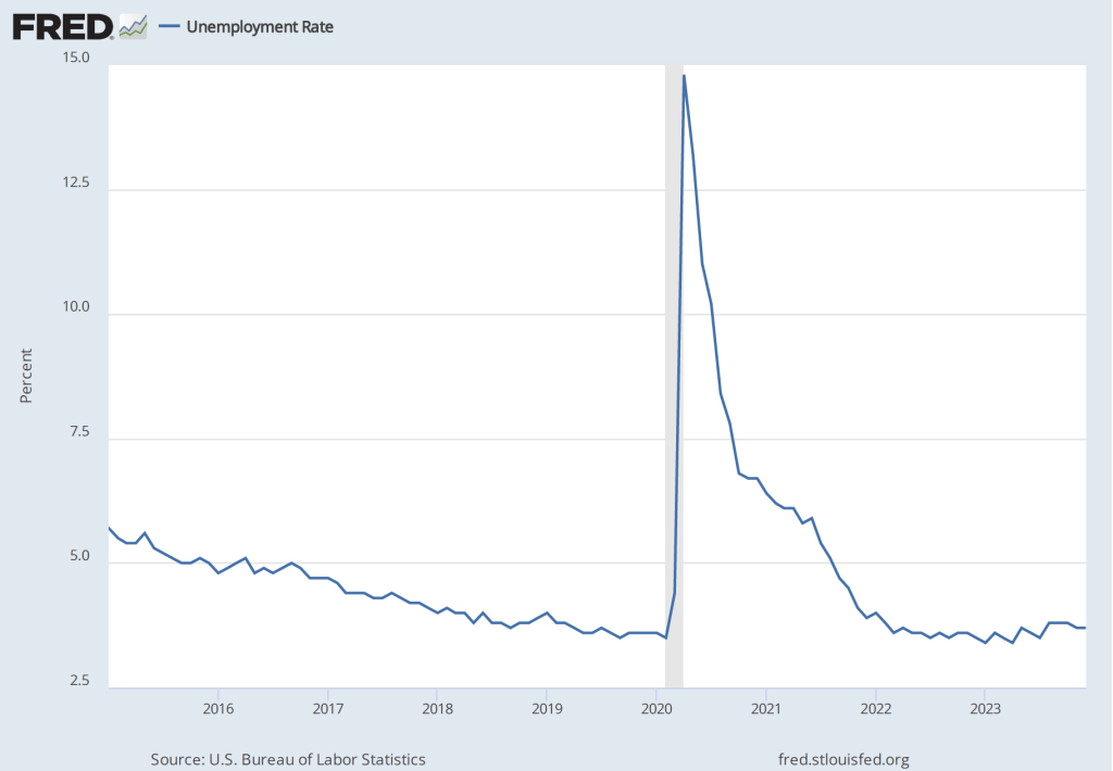
Economists surveyed were also expecting that the unemployment rate—calculated by the BLS from data gathered in the household survey—would increase slightly to 3.8 percent. Instead, it remained constant at 3.7 percent. As the following figure shows, the unemployment rate has been remarkably stable for more than two years and has been below 4.0 percent each month since December 2021. The members of the FOMC expect that the unemployment rate during 2024 will be 4.1 percent, a forcast that will be correct only if the demand for labor declines significantly over the rest of the year.

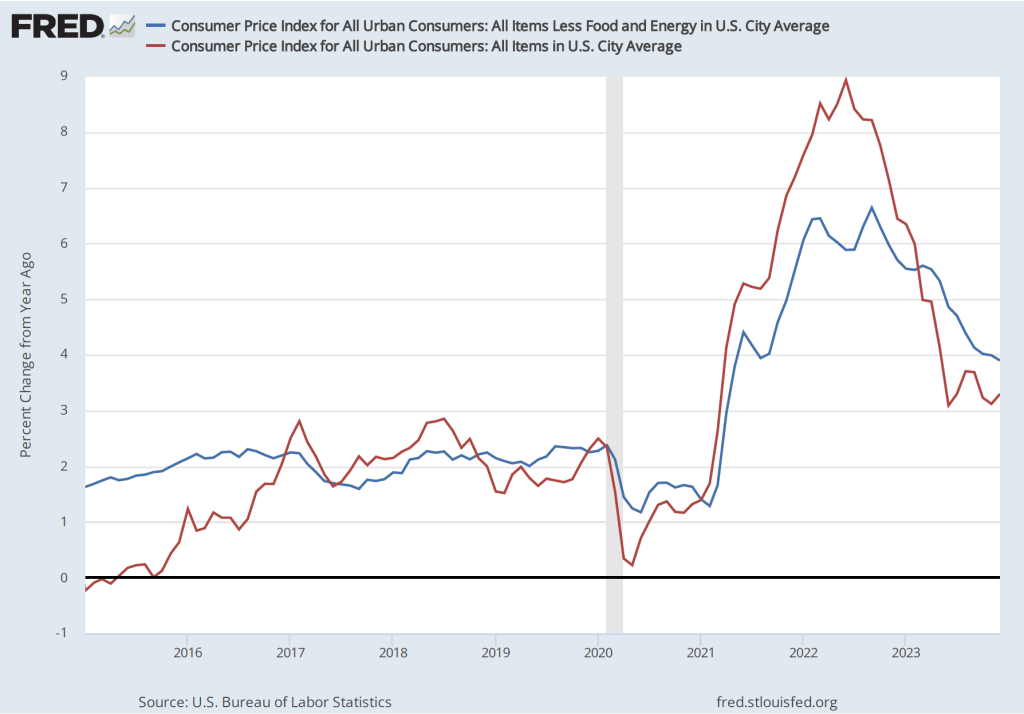
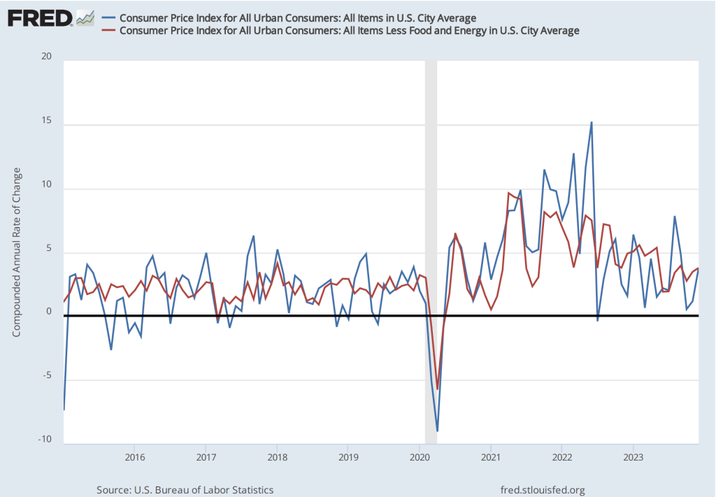
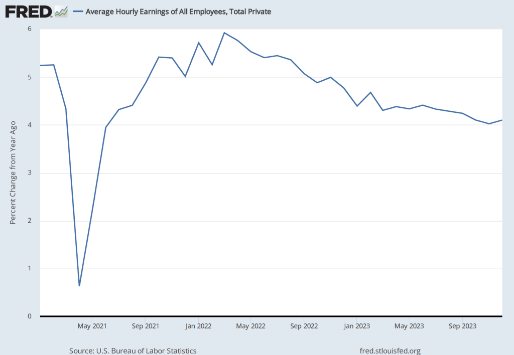
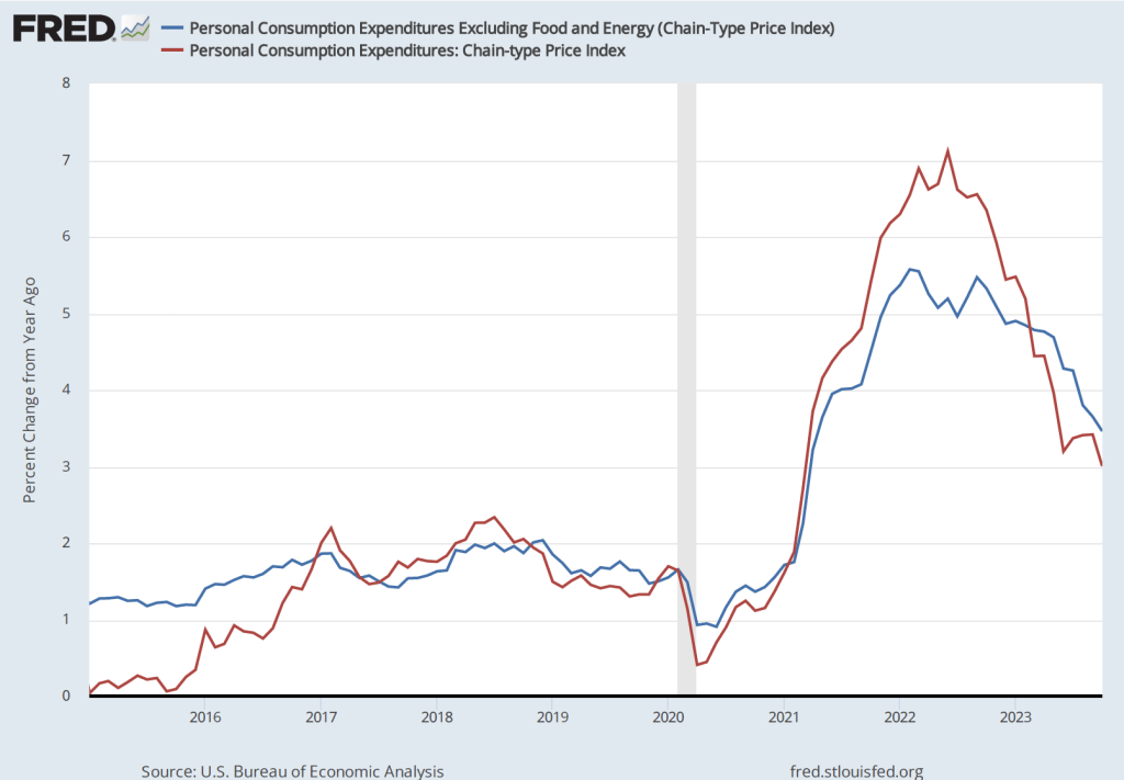
The “Employment Situation Report” also presents data on wages, as measured by average hourly earnings. The growth rate of average hourly earnings, measured as the percentage change from the same month in the previous year, had been slowly declining from March 2022 to October 2023, but has trended upward during the past few months. The growth of average hourly earnings in January 2024 was 4.5 percent, which represents a rise in firms’ labor costs that is likely too high to be consistent with the Fed succeeding in hitting its goal of 2 percent inflation. (Keep in mind, though, as we note in this blog post, changes in average hourly earnings have shortcomings as a measure of changes in the costs of labor to businesses.)

Taken together, the data in today’s “Employment Situation Report” indicate that the U.S. labor market remains very strong. One implication is that the FOMC will almost certainly not cut its target for the federal funds rate at its next meeting on March 19-20. As Fed Chair Jerome Powell noted in a statement to reporters after the FOMC earlier this week: “The Committee does not expect it will be appropriate to reduce the target range until it has gained greater confidence that inflation is moving sustainably toward 2 percent. We will continue to make our decisions meeting by meeting.” (A transcript of Powell’s press conference can be found here.) Today’s employment report indicates that conditions in the labor market may not be consistent with a further decline in price inflation.
It’s worth keeping several things in mind when interpreting today’s report.
- The payroll employment data and the data on average hourly earnings are subject to substantial revisions. This fact was shown in today’s report by the large upward revision in net employment creation in December, as noted earlier in this post.
- A related point: The data reported in this post are all seasonally adjusted, which means that the BLS has revised the raw (non-seasonally adjusted) data to take into account normal fluctuations due to seasonal factors. In particular, employment typically increases substantially during November and December in advance of the holiday season and then declines in January. The BLS attempts to take into account this pattern so that it reports data that show changes in employment during these months holding constant the normal seasonal changes. So, for instance, the raw (non-seasonally adjusted) data show a decrease in payroll employment during January of 2,635,000 as opposed to the seasonally adjusted increase of 353,000. Over time, the BLS revises these seasonal adjustment factors, thereby also revising the seasonally adjusted data. In other words, the BLS’s initial estimates of changes in payroll employment for these months at the end of one year and the beginning of the next should be treated with particular caution.
- The establishment survey data on average weekly hours worked show a slow decline since November 2023. Typically, a decline in hours worked is an indication of a weakening labor market rather than the strong labor market indicated by the increase in employment. But as the following figure shows, the data on average weekly hours are noisy in that the fluctuations are relatively large, as are the revisons the BLS makes to these data over time.

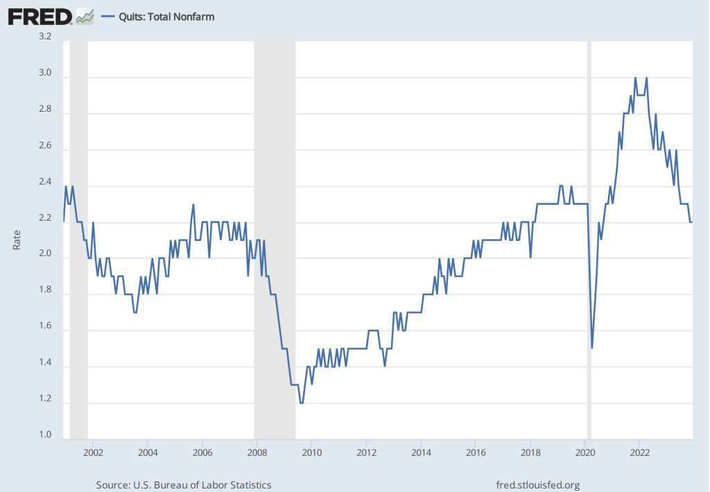
4. In contrast to today’s jobs report, other labor market data seem to indicate that the demand for labor is slowing. For instance, quit rates—or the number of people voluntarily leaving their jobs as a percentage of the total number of people employed—have been declining. As shown in the following figure, the quit rate peaked at 3.0 percent in November 2021 and March 2022, and has declined to 2.2 percent in December 2023—a rate lower than just before the beginning of the Covid–19 pandemic.
Similarly, as the following figure shows, the number of job openings per unemployed person has declined from a high of 2.0 in March 2022 to 1.4 in December 2023. This value is still somewhat higher than just before the beginning of the Covid–19 pandemic.

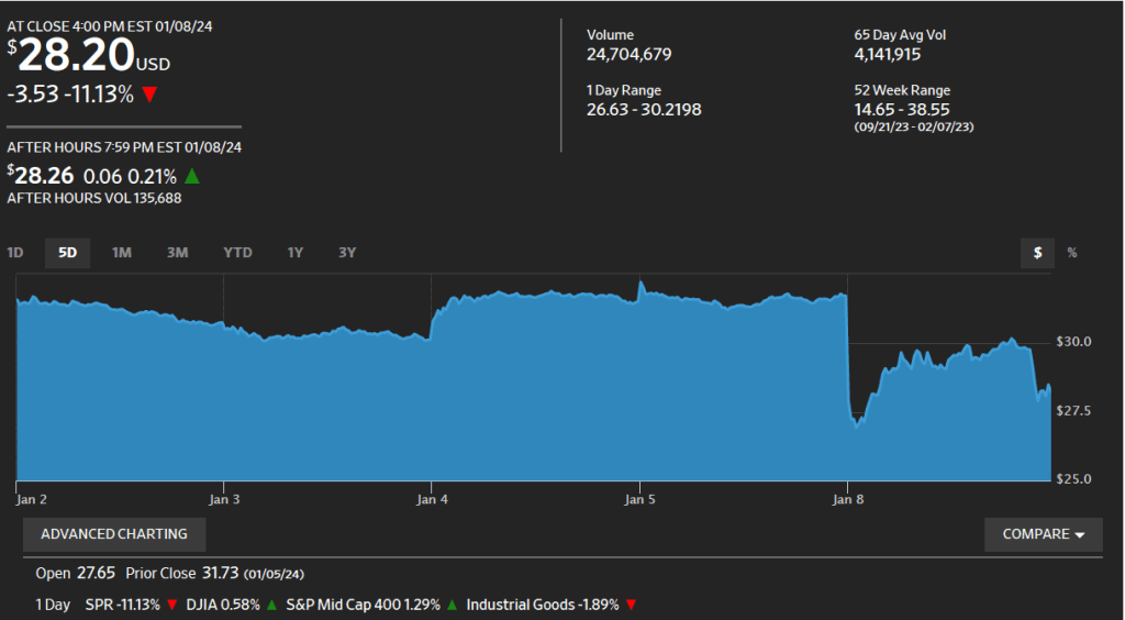
To summarize, recent data on conditions in the labor market have been somewhat mixed. The strong increases in net employment and in average hourly earnings in recent months are in contrast with declining average number of hours worked, a declining quit rate, and a falling number of job openings per unemployed person. Taken together, these data make it likely that the FOMC will be in no hurry to cut its target for the federal funds rate. As a result, long-term interest rates are also likely to remain high in the coming months. The following figure from the Wall Street Journal provides a striking illustration of the effect of today’s jobs report on the bond market, as the interest rate on the 10-year Treasury note rose above 4.0 percent for the first time in more than a month. The interest rate on the 10-year Treasury note plays an important role in the financial system, influencing interest rates on mortgages and corporate bonds.