This morning (May 3), the Bureau of Labor Statistics (BLS) released its “Employment Situation” report for April. The report has two estimates of the change in employment during the month: one estimate from the establishment survey, often referred to as the payroll survey, and one from the household survey. As we discuss in Macroeconomics, Chapter 9, Section 9.1 (Economics, Chapter 19, Section 19.1), many economists and policymakers at the Federal Reserve believe that employment data from the establishment survey provides a more accurate indicator of the state of the labor market than do either the employment data or the unemployment data from the household survey. (The groups included in the employment estimates from the two surveys are somewhat different, as we discuss in this post.)
According to the establishment survey, there was a net increase of 175,000 jobs during April. This increase was well below the increase of 240,000 that economists had forecast in a survey by the Wall Street Journal and well below the net increase of 315,000 during March. The following figure, taken from the BLS report, shows the monthly net changes in employment for each month during the past to years.

As the following figure shows, the net change in jobs from the household survey moves much more erratically than does the net change in jobs in the establishment survey. The net increase in jobs as measured by the household survey fell from 498,000 in March to 25,000 in April.
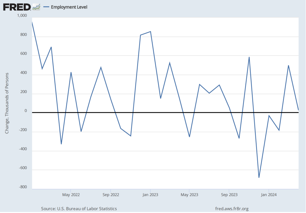
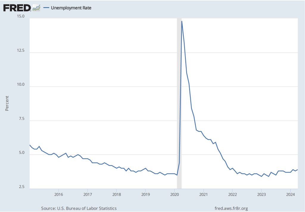
The unemployment rate, which is also reported in the household survey, ticked up slightly from 3.8 percent to 3.9 percent. It has been below 4 percent every month since February 2022.
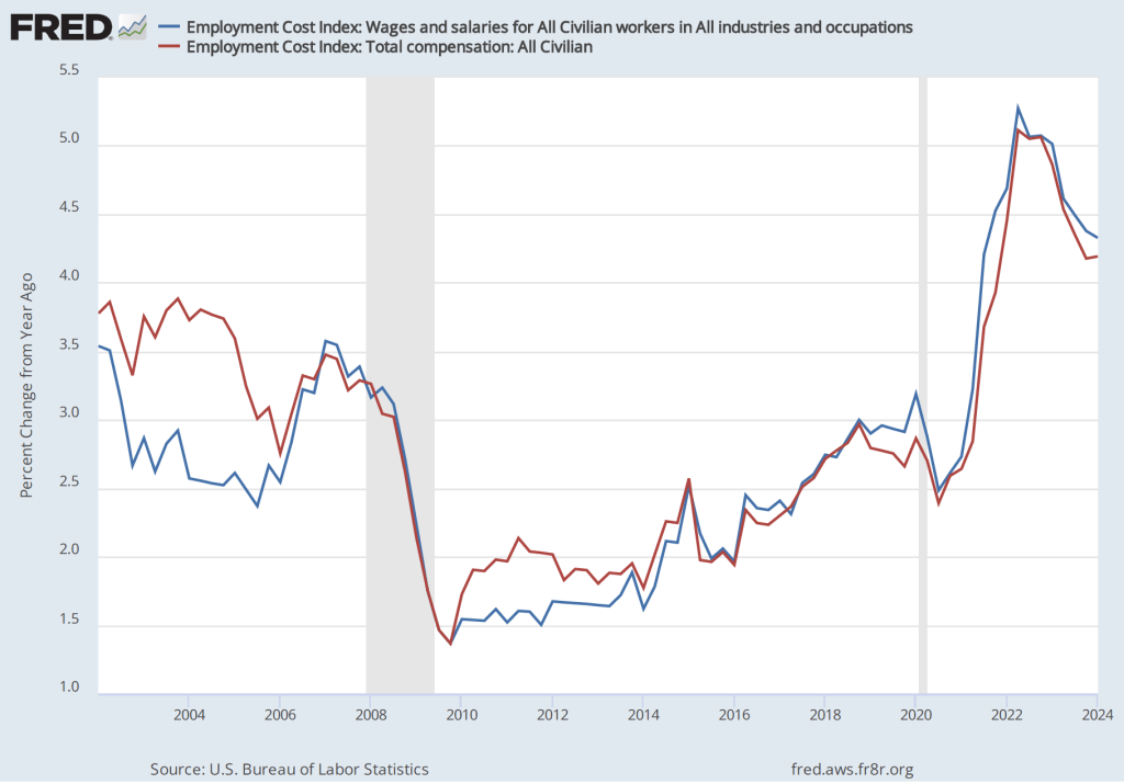
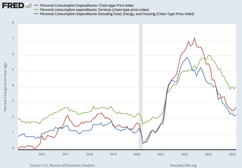
The establishment survey also includes data on average hourly earnings (AHE). As we note in this recent post, many economists and policymakers believe the employment cost index (ECI) is a better measure of wage pressures in the economy than is the AHE. The AHE does have the important advantage that it is available monthly, whereas the ECI is only available quarterly. The following figure show the percentage change in the AHE from the same month in the previous year. The 3.9 percent value for April continues a downward trend that began in February.

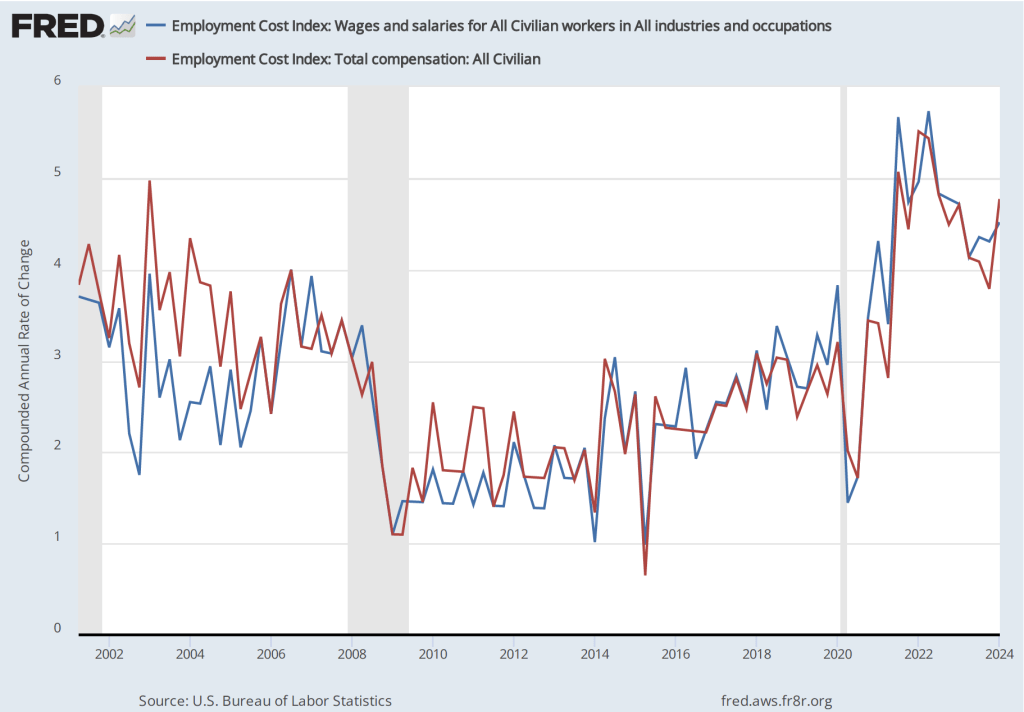
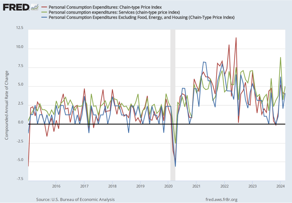
The following figure shows wage inflation calculated by compounding the current month’s rate over an entire year. (The figure above shows what is sometimes called 12-month wage inflation, whereas this figure shows 1-month wage inflation.) One-month wage inflation is much more volatile than 12-month inflation—note the very large swings in 1-month wage inflation in April and May 2020 during the business closures caused by the Covid pandemic.
The 1-month rate of wage inflation of 2.4 percent in April is a significant decrease from the 4.2 percent rate in March, although it’s unclear whether the decline was a sign that the labor market is weakening or reflected the greater volatility in wage inflation when calculated this way.

The macrodata released during the first three months of the year had, by and large, indicated strong economic growth, with the pace of employment increases being particularly rapid. Wages were also increasing at a pace above that during the pre-Covid period. Inflation appeared to be stuck in the range of 3 percent to 3.5 percent, above the Fed’s target inflation rate of 2 percent.
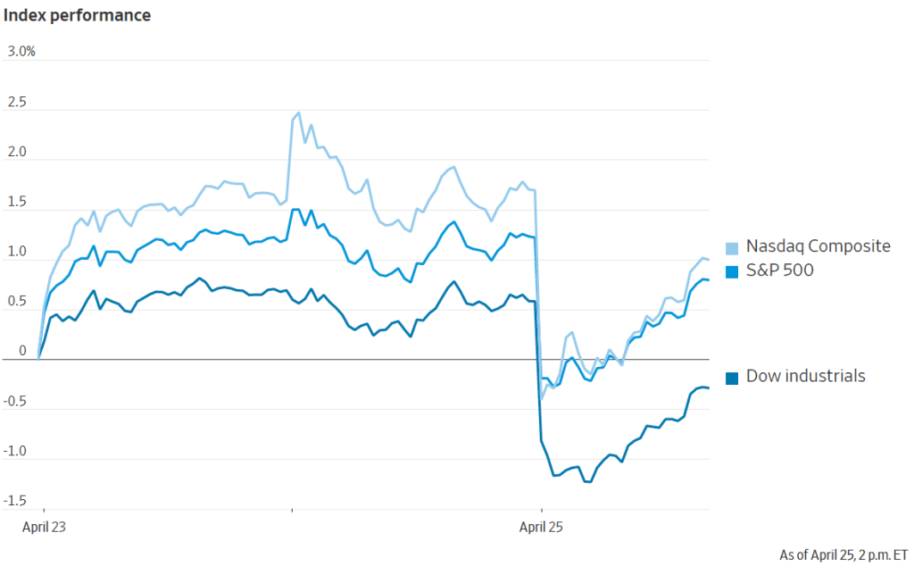
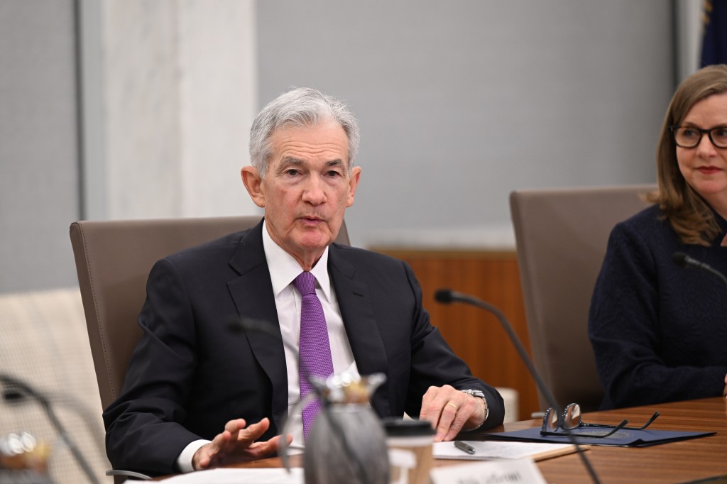
Today’s “Employment Situation” report may be a first indication that growth is slowing sufficiently to allow the inflation rate to fall back to 2 percent. This is the outcome that Fed Chair Jerome Powell indicated in his press conference on Wednesday that he expected to occur at some point during 2024. Financial markets reacted favorably to the release of the report with stock prices jumping and the interest rate on the 10-year Treasury note falling. Many economists and Wall Street analysts had concluded that the Fed’s policy-making Federal Open Market Committee (FOMC) was likely to keep its target for the federal funds rate unchanged until late in the year and might not institute a cut in the target at all this year. Today’s report caused some Wall Street analysts to conclude, as the headline of an article in the Wall Street Journal put it, “Jobs Data Boost Hopes of a Late-Summer Rate Cut.”
This reaction may be premature. Data on employment from the establishment survey can be subject to very large revisions, which reinforces the general caution against putting too great a weight one month’s data. Its most likely that the FOMC would need to see several months of data indicating a slowing in economic growth and in the inflation rate before reconsidering whether to cut the target for the federal funds rate earlier than had been expected.