hubbardobrieneconomics

Latest PCE Report Indicates that Inflation May Be Approaching the Fed’s Target

The result when asking GTP-4o to generate “an image illustrating inflation.”

Inflation, as measured by changes in the personal consumption expenditures (PCE) price index, continued a slow decline that began in March. (The Fed uses annual changes in the PCE price index to evaluate whether it’s meeting its 2 percent annual inflation target.) On August 30, the Bureau of Economic Analysis (BEA) released its “Personal Income and Outlays” report for July, which contains monthly PCE data.

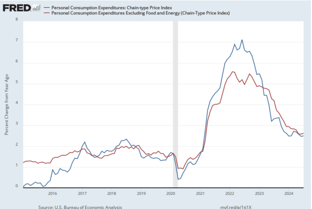
The following figure shows PCE inflation (blue line) and core PCE inflation (red line)—which excludes energy and food prices—for the period since January 2015 with inflation measured as the percentage change in the PCE from the same month in the previous year. Measured this way, in July PCE inflation (the blue line) was 2.5 percent, the same as in June. Core PCE inflation (the red line) in July was 2.6 percent, which was also unchanged from June.

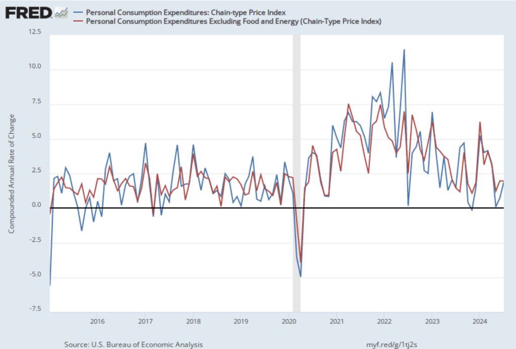
The following figure shows PCE inflation and core PCE inflation calculated by compounding the current month’s rate over an entire year. (The figure above shows what is sometimes called 12-month inflation, while this figure shows 1-month inflation.) Measured this way, PCE inflation rose in July to 1.7 percent from 0.7 percent in July—although higher in July, inflation was below the Fed’s 2 percent target in both months. Core PCE inflation was 2.0 percent in July, which was unchanged from June. These data indicate that inflation has been at or below the Fed’s target for the last three months.

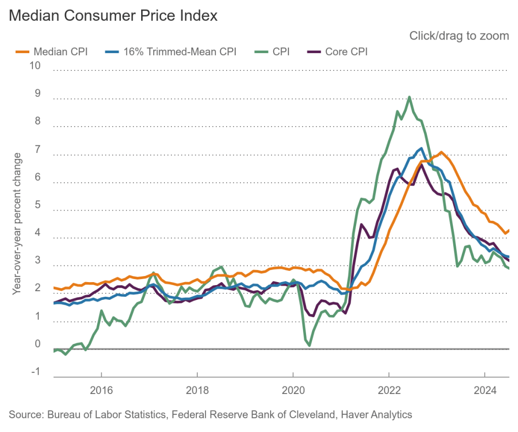
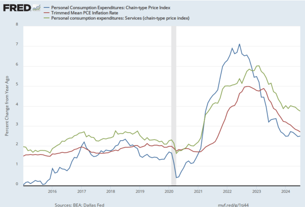
The following figure shows another way of gauging inflation by including the 12-month inflation rate in the PCE (the same as shown in the figure above), inflation measured using only the prices of the services included in the PCE (the green line), and the trimmed mean rate of PCE inflation (the red line). Fed Chair Jerome Powell and other members of the Federal Open Market Committee (FOMC) have said that they are concerned by the persistence of elevated rates of inflation in services. The trimmed mean measure is compiled by economists at the Federal Reserve Bank of Dallas by dropping from the PCE the goods and services that have the highest and lowest rates of inflation. It can be thought of as another way of looking at core inflation by excluding the prices of goods and services that had particularly high or particularly low rates of inflation during the month.

Inflation using the trimmed mean measure was 2.7 percent in July (calculated as a 12-month inflation rate), down only slightly from 2.8 percent in June—and still above the Fed’s target inflation rate of 2 percent. Inflation in services remained high in July at 3.7 percent, although down from 3.9 percent in June.

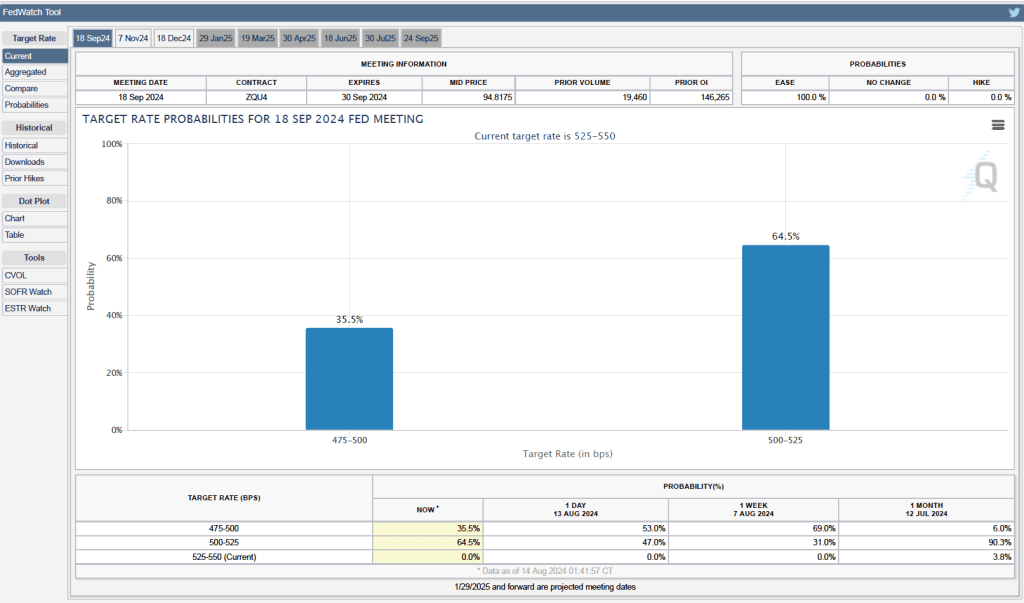
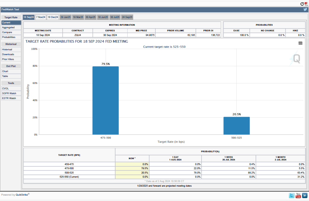
On balance, taking together these various measures, inflation seems on track to return to the Fed’s 2 percent target. As we noted in this earlier post, last week in a speech at the Federal Reserve Bank of Atlanta’s monetary policy symposium in Jackson Hole, Wyoming , Fed Chair Jerome Powell all but confirmed that the the Fed’s policy-maiking Federal Open Market Committee (FOMC) will cut its target for the federal funds rate at its next meeting on September 17-18. There was nothing in this latest PCE report to reduce the likelihood of the FOMC cutting its target at that meeting by an expected 0.25 percent point from a range of 5.25 percent to 5.50 percent to a range of 5.00 percent to 5.25 percent. There also is nothing in the report that would increase likelihood that the committee will cut its target by 0.50 percentage point, as many investors expected following the weak employment report released by the Bureau of labor Statistics (BLS) at the beginning of August. (We discuss this report and the reaction among investors in this post.)

The Continuing Mystery of the Slow Growth in Gross Domestic Income

A fundamental point in macroeconomics is that the value of income and the value of output or production are the same. The Bureau of Economic Analysis (BEA) measures the value of the U.S. economy’s production with gross domestic product (GDP) and the value of total income with gross domestic income (GDI). The two numbers are designed to be equal but because they are compiled from different data, the numbers can diverge. (We discuss GDP and GDI in the Apply the Connection “Was There a Recession during 2022? Gross Domestic Product versus Gross Domestic Income” in Macroeconomics, Chapter 8, Section 8.4 (Economics Chapter 18, Section 18.4).)

The figure above shows that in the past two years the growth rate of real GDP (the green line in the figure) has been significantly different—significantly higher—than the growth rate of GDI (the blue line). Both growth rates are measured as the percentage change from the same quarter in the previous year. Until the fourth quarter of 2022, the two growth rates were roughly similar over the period shown. But for the four quarters beginning in the fourth quarter of 2022, real GDI was flat with a growth rate of 0.0 percent, while real GDP grew at an average annual rate of 1.9 percent during that period. From the fourth quarter of 2023 through the second quarter of 2024, real GDI grew, but at an average annual rate of 1.8 percent, while real GDP was growing at a rate of 3.1 percent. (Some economists prefer to average the growth rates of GDP and GDI, which we show with the red line in the figure.)

In other words, judging by growth in real GDI, the U.S. economy was experiencing something between stagnation and moderate growth, while judging by growth in real GDP, the U.S. economy experiencing moderate to strong growth. There can be differences between GDP and GDI because (1) the BEA uses data on wages, profits, and other types of income to measure GDI, and (2) the errors in these data can differ from the errors in data on production and spending used to estimate GDP.

Jason Furman, chair of the Council of Economic Advisers under President Barack Obama, has suggested that a surge in immigration may explain why GDI growth has lagged GDP growth. As we discuss in this blog post, the Census Bureau may have been underestimating the number of immigrants who have entered the United States in recent years. The Congressional Budget Office (CBO) estimates that there are actually 6 million more people living in the United States in 2024 than the Census Bureau estimates because the bureau has underestimated the number of immigrants.

Compared to the native-born population, immigrants are disproportionately in the prime working ages of 25 to 54 and are therefore more likely to be in the labor force. It seems plausible—although so far as we know, the point hasn’t been documented—that the value of production resulting from the work of uncounted (in the census estimates) immigrants is more likely to be included in GDP than the income they are paid is to be counted in GDI. The result could explain at least part of the discrepancy between GDP and GDI that we’ve seen in the past two years. But while this factor affects the levels of GDP and GDI, it’s not clear that it affects the growth rates of GDP and GDI. The number of uncounted immigrants would have to be increasing over time for the growth rate of GDI to be reduced relative to the growth rate of GDP.

This episode may demonstrate the need for Congress to provide the BEA staff with resources they would need to do the work required to reconcile GDP estimates with GDI estimates.

Glenn’s Interview with Jim Pethokoukis

Glenn discusses Fed policy, the state of the U.S economy, economic growth, China in the world economy, industrial policy, protectionism, and other topics in this episode of the Political Economy podcast from the American Enterprise Institute.

https://podcasts.apple.com/us/podcast/glenn-hubbard-a-pro-growth-policy-agenda/id589914386?i=1000665131415

Did Taylor Swift’s Fans Break Economics?

Image generated by GTP-4o of a woman singer performing at a concert.

The answer to the question in the title is “yes” according to a column by James Mackintosh in the Wall Street Journal. In the Apply the Concept “Taylor Swift Tries to Please Fans and Make Money,” in Chapter 11 of Microeconomics, we discussed how for her The Eras Tour, Taylor Swift reserved more than half of the concert tickets for her “verified fans.” The tickets sold to verified fans for an average price of $250.

On the resale market, prices of the tickets soared to $1,000 or more. Yet only about 5 percent of tickets purchased by verified fans were resold. Mackintosh’s wife and “eldest offspring” were in in the other 95 percent—they had purchased their tickets at a low price but wouldn’t resell them at a much higher price. Moreover—and this is where Mackintosh sees economics as breaking—if they didn’t already have the tickets they wouldn’t have bought them at the current high price.

Not being willing to buy something at a price you wouldn’t sell it for is inconsistent behavior because it ignores a nonmonetary opportunity cost. (As we discuss in Chapter 10, Section 10.4.) If Mackintosh’s wife won’t sell her ticket for $1,000, she incurs a $1,000 opportunity cost, which is the amount she gives up by not selling the ticket. The two alternatives—either paying $1,000 for a ticket or not receiving $1,000 by declining to sell a ticket—amount to exactly the same thing.

Mackintosh recognizes that the actions of his wife and offspring reflect what he calls a “mental bias,” which he correctly labels the endowment effect: The tendency to be unwilling to sell something you already own even if you are offered a price greater than the price you would be willing to buy the thing for if you didn’t already own it.

As we discuss in Chapter 10, the endowment effect is one of a number of results from behavioral economics, which is the study of situations in which people make choices that don’t appear to be economically rational. So, Mackintosh’s family—and other Swifties—didn’t break economics. Instead, they demonstrated one of the results of behavioral economics.

Fed Chair Powell Indicates that Rate Cuts Will Begin Soon

Photo of Federal Reserve Chair Jerome Powell from federalreserve.gov

Federal Reserve chairs often take the opportunity of the Kansas City Fed’s annual monetary policy symposium held in Jackson Hole, Wyoming to provide a summary of their views on monetary policy and on the state of the economy. In speeches, Fed chairs are careful not to preempt decisions of the Federal Open Market Committee (FOMC) by stating that policy changes will occur that the committee hasn’t yet agreed to. In his speech at Jackson Hole on Friday (August 23), Powell came about as close as Fed chairs ever do to announcing a policy change in a speech.

In the speech, Powell indicated that: “The time has come for policy to adjust. The direction of travel is clear, and the timing and pace of rate cuts will depend on incoming data, the evolving outlook, and the balance of risks.” The statement is effectively an announcement that the FOMC will reduce its target for the federal funds rate at its next meeting on September 17-18. By referring to “the timing and pace of rate cuts,” Powell was indicating that the FOMC was likely to eventually reduce its target for the federal funds rate well below its current 5.25 percent to 5.50 percent, although the reductions will be spread out over a number of meetings.

The minutes of the FOMC’s last meeting on July 30-31 were released on August 21. The minutes stated that: “The vast majority [of committee members] observed that, if the data continued to come in about as expected, it would likely be appropriate to ease policy at the next meeting.” The apparent consensus at the July meeting that the target for the federal funds rate should be reduced at the September meeting was likely the key reason why Powell was so forthright in his speech.

In his speech, Powell summarized his views on the reasons that inflation accelerated in 2021 and why it has slowly declined since reaching a peak in the summer of 2022:

“[The analysis of events that Powell supports] attributes much of the increase in inflation to an extraordinary collision between overheated and temporarily distorted demand and constrained supply. While researchers differ in their approaches and, to some extent, in their conclusions, a consensus seems to be emerging, which I see as attributing most of the rise in inflation to this collision. All told, the healing from pandemic distortions, our efforts to moderate aggregate demand, and the anchoring of expectations have worked together to put inflation on what increasingly appears to be a sustainable path to our 2 percent objective.”

As he has over the past three years, Powell emphasized the importance of expectations having remained “anchored,” meaning that households and firms continued to expect that the annual inflation rate would return to 2 percent, even when the current inflation rose far above that rate. We discuss how expectations of inflation affect the current inflation rate in Macroeconomics, Chapter 17 (Economics, Chapter 27).

Where Did 818,000 Jobs Go?

Image of “people attending a job fair” generated by GTP-4o

On Wednesday, August 21, the Bureau of Labor Statistics (BLS) issued revised estimates of the increase in employment, as measured by the establishment survey, over the period from April 2023 through March 2024. The BLS had initially estimated that on average during that period net employment had increased by 242,000 jobs per month. The revision lowered this estimate by 28 percent to an average of only 174,000 net new jobs created per month. The difference between those two monthly averages means that the U.S. economy had generated a total of 818,000 fewer jobs during that period.

Why does the BLS have to revise its employment estimates? As we discuss in Macroeonomics, Chapter 9, Section 9.1 (Economics, Chapter 19, Section 19.1) the initial estimates that the BLS issues each month in its “Employment Situation” reports are based on a sample of 300,000 establishments. The monthly data also rely on estimates of the number of employees at establishments that opened or closed during the month and on employment changes at establishments that failed to respond to the survey. In August of each year, the BLS issues revised employment estimates based on state unemployment insurance tax records, which are much more comprehensive than the original sample of establishments because nearly all employers are included.

Although this year’s revision is particularly large in absolute terms—the largest since 2009—it still represents only about 0.5 percent of the more than 158 million people employed in the U.S. economy. How will this revision affect the decision by the Federal Open Market Committee (FOMC) at its next meeting on September 17-18 to cut or maintain its target for the federal funds rate? The members of the committee were probably not surprised by the downward revision in the employment estimates, although they may have anticipated that the revision would be smaller. In five of the past six years, the BLS has revised its estimates of payroll employment downward in its annual benchmark revision.

In his press conference following the June 12 FOMC meeting, Fed Chair Jerome Powell observed that “you have payroll jobs still coming in strong, even though, you know, there’s an argument that they may be a bit overstated.” (Note that FOMC members don’t receive the data in BLS reports until the reports are publicly released.) As we noted in this recent post, even before the BLS revised its employment estimates downward, recent monthly increases were below the level likely needed to keep up with population growth—so-called breakeven employment growth. There was already a high likelihood that the FOMC intended to cut its target for the federal funds rate at its September meeting. The substantial downward revision in the employment data makes a cut nearly a certainty.

Chair Powell is scheduled to give a speech on Friday morning at the Kansas City Fed’s annual monetary policy symposium held in Jackson Hole, Wyoming. During that speech, he’s likely to give his reaction to the revised employment data—and the state of the labor market more generally.

CPI Inflation Is Lowest Since March 2021

Photo courtesy of Lena Buonanno

Today (August 14), the Bureau of Labor Statistics (BLS) released its monthly report on the consumer price index (CPI), which showed inflation falling below 3 percent for the first time since March 2021.

As the following figure shows, the inflation rate for July measured by the percentage change in the CPI from the same month in the previous month—headline inflation (the blue line)—was 2.9 percent down from 3.0 percent in June. Core inflation (the red line)—which excludes the prices of food and energy—was 3.2 percent in July, down from 3.3 percent in June.

As the following figure shows, if we look at the 1-month inflation rate for headline and core inflation—that is the annual inflation rate calculated by compounding the current month’s rate over an entire year—we see an increase in the inflation rate in July, but the increase is from the very low levels in June. Headline inflation (the blue line) increased from –0.7 percent in June (which means that consumer price actually fell that month) to 1.9 percent in July. Core inflation (the red line) increased from 0.8 percent in June to 2.o percent in July. Overall, we can say that, taking 1-month and 12 month inflation together, the U.S. economy seems on course for a soft landing—with the annual inflation rate returning to the Fed’s 2 percent target without the economy being pushed into a recession. (Note, though, that the Fed uses the personal consumption expenditures (PCE) price index, rather than the CPI in evaluating whether it is hitting its 2 percent inflation target.)

Federal Reserve Chair Jerome Powell and his colleagues on the policy-making Federal Open Market Committee (FOMC) have been closely following inflation in the price of shelter. The price of “shelter” in the CPI, as explained here, includes both rent paid for an apartment or house and “owners’ equivalent rent of residences (OER),” which is an estimate of what a house (or apartment) would rent for if the owner were renting it out. OER is included to account for the value of the services an owner receives from living in an apartment or house.

As the following figure shows, inflation in the price of shelter has been a significant contributor to headline inflation. The blue line shows 12-month inflation in shelter and the red line shows 1-month inflation in shelter. Twelve-month inflation in shelter continued its decline that began in the spring of 2023, falling from 5.1 percent in June to 5.0 percent July. One-month inflation in shelter—which is much more volatile than 12-month inflation in shelter—increased from 2.1 percent in June to 4.6 percent in July. The value for 1-month inflation in shelter may concern the members of the FOMC, but the continuing decline in in the less volatile 12-month inflation in shelter provides some reassurance that inflation in shelter is likely continuing to decline.

Finally, in order to get a better estimate of the underlying trend in inflation, some economists look at median inflation and trimmed mean inflation. Median inflation is calculated by economists at the Federal Reserve Bank of Cleveland and Ohio State University. If we listed the inflation rate in each individual good or service in the CPI, median inflation is the inflation rate of the good or service that is in the middle of the list—that is, the inflation rate in the price of the good or service that has an equal number of higher and lower inflation rates. Trimmed mean inflation drops the 8 percent of good and services with the higherst inflation rates and the 8 percent of goods and services with the lowest inflation rates.

As the following figure (from the Federal Reserve Bank of Cleveland) shows, median inflation (the brown line) ticked up slightly from 4.2 percent in June to 4.3 percent in July. Trimmed mean inflation (the blue line) was unchanged in July at 3.3 percent. One conclusion from these data is that headline and core inflation may be somewhat understating the underlying rate of inflation.

For the past few weeks investores in financial markets have been expecting that recent inflation and employment data will lead the FOMC to cut its target for the federal funds at its next meeting on Septembe 17-18 .

Futures markets allow investors to buy and sell futures contracts on commodities–such as wheat and oil–and on financial assets. Investors can use futures contracts both to hedge against risk—such as a sudden increase in oil prices or in interest rates—and to speculate by, in effect, betting on whether the price of a commodity or financial asset is likely to rise or fall. (We discuss the mechanics of futures markets in Chapter 7, Section 7.3 of Money, Banking, and the Financial System.) The CME Group was formed from several futures markets, including the Chicago Mercantile Exchange, and allows investors to trade federal funds futures contracts. The data that result from trading on the CME indicate what investors in financial markets expect future values of the federal funds rate to be. The following chart from the CME’s FedWatch Tool shows the current values from trading of federal funds futures.

The probabilities in the chart reflect investors’ predictions of what the FOMC’s target for the federal funds rate will be after the committee’s September meeting. The chart indicates that investors assign a probability of 35.5 percent to the FOMC cutting its target range for the federal funds rate by 0.50 percentage point from the current 5.25 prcent to 5.50 percent to 4.75 percent to 5.25 percent. Investors assign a much larger probability—64.5 percent—to the FOMC cutting its target range for the federal funds rate by 0.25 percentage point to 5.00 percent to 5.25 percent.

It would most likely require the next BLS “Employment Situation” report—which is scheduled for release on September 6—to show unexpected weakness for the FOMC to cut its target for the federal funds rate by more than 0.25 percentage point.

Stock Prices Rise and Bond Prices Fall with Decline in Initial Jobless Claims

Over the first past few days, the stock and bond markets have gone through substantial swings as investors try to determine whether the U.S. economy is likely to move into a recession soon. (We discussed here the most recent BLS “Employment Situation” report, which was surprisingly weak.)

It’s difficult to determine with certainty why on a particular day stock and bond prices fluctuate. The following two figures from the Wall Street Journal show movements this morning (August 8) in stock prices and bond yields. (Recall that bond yields rise when bond prices fall, a point we discuss in the Appendix to Chapter 6 of Macroeconomics (Chapter 8 of Economics).)

Rising stock prices and falling bond prices (rising bond yields) can be an indication that investors are more optimistic that the U.S. economy will avoid a recession. In a recession, profits decline, which is bad for stock prices. And in a recession, interest rates typically fall both because the Federal Reserve cuts it target range for the federal funds rate and because household and firms borrow less, which reduces the demand for loanable funds. Accordingly, most analysts are attributing the movements in stock and bond prices this morning to investors becoming more optimistic that the U.S. economy will avoid a recession.

Because of the level of uncertainty about the future path of the economy, investors are following very closely the release of new macroeconomic data. The Wall Street Journal and other business publications attributed the increase in investor optimism this morning to the U.S. Employment and Training Administration releasing at 8:30 a.m. its latest report on initial claims for unemployment insurance. The headline in the Wall Street Journal was: “Stocks Rise on Claims Data.” Similalry, the headline on bloomberg.com was: “Stocks Get Relief Rally after Jobless Claims Data.”

What are jobless claims? The first step when you lose a job and wish to receive government unemployment insurance payments is to file a claim, which starts the process by which an agency of the state government determines whether you are eligible to receive unemployment insurance payments.

The data on initial jobless claims are released weekly. As the following figure shows, there is a lot of volatility in this data series. The latest data were favorable—which is thought to have caused the increase in stock prices and decline in bond prices—because new claims declined by 17,000 this week. But the series is so volatile that drawing conclusions from weekly changes seems unwarranted. For instance, the figure shows that weekly claims surged during the summer of 2023, although employment and production continued to expand during that period.

So it appears that people trading in stock and bond markets this morning are overreacting to this macrodata release. But explanations of why stock and bonds prices move as they do over a short period of time often turnout in hindsight to have been incorrect. It may well be the case that investors are acting as they are this morning for reasons that are, in fact, unrelated to the data on jobless claims.

Solved Problem: If Employment and Unemployment Both Increase, What Happens to the Unemployment Rate?

Supports: Macroeconomics, Chapter 9, Economics, Chapter 19, and Essentials of Economics, Chapter 13.

Image generated by GTP-4o.

In its “Employment Situation” report for July 2024, the Bureau of Labor Statistics (BLS) stated that according to the household survey the total number of people employed, the total number of people unemployed, and the unemployment rate all increased. Would we expect this result to always hold? That is, in a month in which both the total number of people employed and the total number of people unemployed increased will the unemployment rate always increase? Briefly explain.

Solving the Problem
Step 1: Review the chapter material. This problem is about calculating the unemployment rate, so you may want to review Chapter 9, Section 9.1, “Measuring the Unemployment Rate, the Labor Force Participation Rate, and the Employment-Population Ratio.”

Step 2: Answer the question by explaining whether we can be certain what happens to the unemployment rate in a month in which both the total number of people employed and the total number of people unemployed increased. The unemployment rate is equal to the number of people unemployed divided by the number of people in the labor force (multiplied by 100). The labor force equals the sum of the number of people employed and the number of people unemployed.

Suppose, for example, that the unemployment rate in the previous month was 4 percent. If both the number of people employed and the number of people unemployed increase, the unemployment rate will increase if the increase in the number of people unemployed as a percentage of the increase in the labor force is greater than 4 percent. The unemployment rate will decrease if the increase in the number of people unemployed as a percentage of the increase in the labor force is less than 4 percent.

Consider a simple numerical example. Suppose that in the previous month there were 96 people employed and 4 people unemployed. In that case, the unemployment rate will be (4/(96 + 4)) x 100 = 4.0%.

Suppose that during the month the number of people employed increases by 30 and the number of people unemployed increases by 1. In that case, there are now 126 people employed and 5 people unemployed. The unemployment rate will have fallen from 4.0% to (5/(126 + 5)) x 100 = 3.8%.

Now suppose that the number of people employed increased by 30 and the number of people unemployed increases by 3. The unemployment will have risen from 4.0% to (7/(126 + 7)) x 100 = 5.3%.

We can conclude that what happened in July 2024 need not always happen. If both the total number of people employed and the total number of people unemployed increased during a given month, we can’t be sure whether the unemployment rate has increased or decreased.

Unexpectedly Weak Employment Report; Beware the Sahm Rule?

Earlier this week, as we discussed in this blog post, the Federal Reserve’s policy-making Federal Open Market Committee (FOMC) voted to leave its target for the federal funds rate unchanged. In his press conference following the meeting, Fed Chair Jerome Powell stated that: “Overall, a broad set of indicators suggests that conditions in the labor market have returned to about where they stood on the eve of the pandemic—strong but not overheated.”

This morning (August 2), the Bureau of Labor Statistics (BLS) released its “Employment Situation” report (often referred to as the “jobs report”) for July, which indicates that the labor market may be weaker than Powell and the other members of the FOMC believed it to be when they decided to leave their target for the federal funds rate unchanged.

The jobs report has two estimates of the change in employment during the month: one estimate from the establishment survey, often referred to as the payroll survey, and one from the household survey. As we discuss in Macroeconomics, Chapter 9, Section 9.1 (Economics, Chapter 19, Section 19.1), many economists and policymakers at the Federal Reserve believe that employment data from the establishment survey provides a more accurate indicator of the state of the labor market than do either the employment data or the unemployment data from the household survey. (The groups included in the employment estimates from the two surveys are somewhat different, as we discuss in this post.)

According to the establishment survey, there was a net increase of 114,000 jobs during July. This increase was below the increase of 175,000 to 185,000 that economists had forecast in surveys by the Wall Street Journal and bloomberg.com. The following figure, taken from the BLS report, shows the monthly net changes in employment for each month during the past two years.

The previously reported increases in employment for April and May were revised downward by 29,000 jobs. (The BLS notes that: “Monthly revisions result from additional reports received from businesses and government agencies since the last published estimates and from the recalculation of seasonal factors.”) As we’ve discussed in previous posts (most recently here), downward revisions to the payroll employment estimates are particularly likely at the beginning of a recession, although this month’s adjustments were relatively small.

As the following figure shows, the net change in jobs from the household survey moves much more erratically than does the net change in jobs in the establishment survey. The net change in jobs as measured by the household survey declined from 116,000 in June to 67,000 in June. So, in this case the direction of change in the two surveys was the same—a decline in the increase in the number of jobs.

As the following figure shows, the unemployment rate, which is also reported in the household survey, increased from 4.1 percent to 4.3 percent—the highest unemployment rate since October 2021. Although still low by historical standards, July was the fifth consecutive month in which the unemployment rate increased. It is also higher than the unemployment rate just before the pandemic. The unemployment rate was below 4 percent most months from mid-2018 to early 2020.

Some economists and policymakers have been following the Sahm rule, named after Claudia Sahm Chief Economist for New Century Advisors and a former Fed economist. The Sahm rule, as stated on the site of the Federal Reserve Bank of St. Louis is: “Sahm Recession Indicator signals the start of a recession when the three-month moving average of the national unemployment rate (U3 [measure]) rises by 0.50 percentage points or more relative to the minimum of the three-month averages from the previous 12 months.” The following figure shows the values of this indicator dating back to March 1949.

So, according to this indicator, the U.S. economy is now at the start of a recession. Does that mean that a recession has actually started? Not necessarily. As Sahm stated in an interview this morning, her indicator is a historical relationship that may not always hold, particularly given how signficantly the labor market has been affected during the last four years by the pandemic.

As we noted in a post earlier this week, investors who buy and sell federal funds futures contracts assigned a probability of 11 percent that the FOMC would cut its target for the federal funds rate by 0.50 percentage point at its next meeting. (Investors in this market assigned a probability of 89 percent that the FOMC would cut its target by o.25 percentage point.) Today, investors dramatically increased the probability to 79.5 percent of a 0.50 cut in the federal funds rate target, as shown in this figure from the CME site.

Investors on the stock market appear to believe that the probability of a recession beginning before the end of the year has increased, as indicated by sharp declines today in the stock market indexes.

The next scheduled FOMC meeting isn’t until September 17-18. The FOMC is free to meet in between scheduled meetings but doing so might be interpreted as meanng that economy is in crisis, which is a message the committee is unlikely to want to send. It would likely take additional unfavorable reports on macro data for the FOMC not to wait until September to take action on cutting its target for the federal funds rate.