
Join authors Glenn Hubbard and Tony O’Brien as they discuss how core economic principles illuminate two of the most pressing policy debates facing the economy today: tariffs and artificial intelligence. Drawing on a recent Supreme Court decision striking down broad tariff increases, Hubbard and O’Brien explain why economists view tariffs as taxes, who ultimately bears their burden, and how trade policy uncertainty shapes business decisions, inflation, and economic growth—bringing textbook concepts like tax incidence, intermediate goods, and GDP measurement vividly to life. The conversation then turns to AI, where they cut through market hype and dire predictions to place generative AI in historical context as a general‑purpose technology, comparing it to past innovations that transformed jobs without eliminating work. Along the way, they explore how AI can both substitute for and complement labor, why fears of mass unemployment are likely overstated, and what economists can—and cannot yet—say about AI’s long‑run effects on productivity, profits, and the labor market.
Tag: tariffs
Solved Problem: Using the Demand and Supply Model to Analyze the Effects of a Tariff on Televisions
Supports: Microeconomics, Macroeconomics, Economics, and Essentials of Economics, Chapter 4, Section 4.4

Image generated by ChapGPT
The model of demand and supply is useful in analyzing the effects of tariffs. In Chapter 9, Section 9.4 (Macroeconomics, Chapter 7, Section 7.4) we analyze the situation—for instance, the market for sugar—when U.S. demand is a small fraction of total world demand and when the U.S. both produces the good and imports it.
In this problem, we look at the television market and assume that no domestic firms make televisions. (A few U.S. firms assemble limited numbers of televisions from imported components.) As a result, the supply of televisions consists entirely of imports. Beginning in April, the Trump administration increased tariff rates on imports of televisions from Japan, South Korea, China, and other countries. Tariffs are effectively a tax on imports, so we can use the analysis in Chapter 4, Section 4.4, “The Economic Effect of Taxes” to analyze the effect of tariffs on the market for televisions.
- Use a demand and supply graph to illustrate the effect of an increased tariff on imported televisions on the market for televisions in the United States. Be sure that your graph shows any shifts of the curves and the equilibrium price and quantity of televisions before and after the tariff increase.
- An article in the Wall Street Journal discussed the effect of tariffs on the market for used goods. Use a second demand and supply graph to show the effect of a tariff on imports of new televisions on the market in the United States for used televisions. Assume that no used televisions are imported and that the supply curve for used televisions is upward sloping.
Solving the Problem
Step 1: Review the chapter material. This problem is about the effect of a tariff on an imported good on the domestic market for the good. Because a tariff is a like a tax, you may want to review Chapter 4, Section 4.4, “The Economic Effect of Taxes.”
Step 2: Answer part a. by drawing a demand and supply graph of the market for televisions in the United States that illustrates the effect of an increased tariff on imported televisions. The following figure shows that a tariff causes the supply curve of televisions to shift up from S1 to S2. As a result, the equilibrium price increases from P1 to P2, while the equilibrium quantity falls from Q1 to Q2.
Step 2: Answer part b. by drawing a demand and supply graph of the market for used televisions in the United States that illustrates the effect on that market of an increased tariff on imports of new televisions. Although the tariff on imported televisions doesn’t directly affect the market for used televisions, it does so indirectly. As the article from the Wall Street Journal notes, “Today, in the tariff era, demand for used goods is surging.” Because used televisions are substitutes for new televisions, we would expect that an increase in the price of new televisions would cause the demand curve for used televisions to shift to the right, as shown in the following figure. The result will be that the equilibrium price of used televisions will increase from P1 to P2, while the equilibrium quantity of used televisions will increase from Q1 to Q2.
To summarize: A tariff on imports of new televisions increases the price of both new and used televisions. It decreases the quantity of new televisions sold but increases the quantity of used televisions sold.
NEW! 11-07-25- Podcast – Authors Glenn Hubbard & Tony O’Brien discuss Tariffs, AI, and the Economy
Glenn Hubbard and Tony O’Brien begin by examining the challenges facing the Federal Reserve due to incomplete economic data, a result of federal agency shutdowns. Despite limited information, they note that growth remains steady but inflation is above target, creating a conundrum for policymakers. The discussion turns to the upcoming appointment of a new Fed chair and the broader questions of central bank independence and the evolving role of monetary policy. They also address the uncertainty surrounding AI-driven layoffs, referencing contrasting academic views on whether artificial intelligence will complement existing jobs or lead to significant displacement. Both agree that the full impact of AI on productivity and employment will take time to materialize, drawing parallels to the slow adoption of the internet in the 1990s.
The podcast further explores the recent volatility in stock prices of AI-related firms, comparing the current environment to the dot-com bubble and questioning the sustainability of high valuations. Hubbard and O’Brien discuss the effects of tariffs, noting that price increases have been less dramatic than expected due to factors like inventory buffers and contractual delays. They highlight the tension between tariffs as tools for protection and revenue, and the broader implications for manufacturing, agriculture, and consumer prices. The episode concludes with reflections on the importance of ongoing observation and analysis as these economic trends evolve.
Pearson Economics · Hubbard OBrien Economics Podcast – 11-06-25 – Economy, AI, & Tariffs
PCE Inflation Is Steady, but Still Above the Fed’s Target
On August 29, the Bureau of Economic Analysis (BEA) released data for July on the personal consumption expenditures (PCE) price index as part of its “Personal Income and Outlays” report. The Fed relies on annual changes in the PCE price index to evaluate whether it’s meeting its 2 percent annual inflation target.
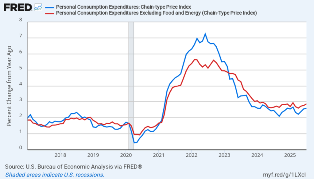
The following figure shows headline PCE inflation (the blue line) and core PCE inflation (the red line)—which excludes energy and food prices—for the period since January 2017, with inflation measured as the percentage change in the PCE from the same month in the previous year. In July, headline PCE inflation was 2.6 percent, unchanged from June. Core PCE inflation in July was 2.9 percent, up slightly from 2.8 percent in June. Headline PCE inflation and core PCE inflation were both equal to what economists surveyed had forecast.
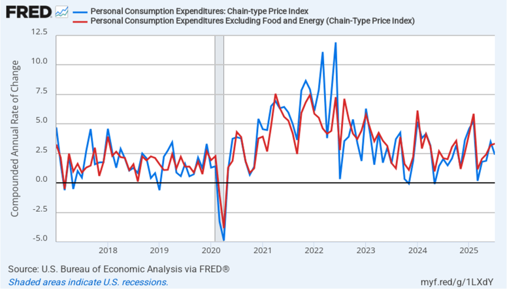
The following figure shows headline PCE inflation and core PCE inflation calculated by compounding the current month’s rate over an entire year. (The figure above shows what is sometimes called 12-month inflation, while this figure shows 1-month inflation.) Measured this way, headline PCE inflation fell from 3.5 percent in June to 2.4 percent in July. Core PCE inflation increased slightly from 3.2 percent in June to 3.3 percent in July. So, both 1-month PCE inflation estimates are above the Fed’s 2 percent target, with 1-month core PCE inflation being well above target. The usual caution applies that 1-month inflation figures are volatile (as can be seen in the figure), so we shouldn’t attempt to draw wider conclusions from one month’s data. In addition, these data may reflect higher prices resulting from the tariff increases the Trump administration has implemented. Once the one-time price increases from tariffs have worked through the economy, inflation may decline. It’s not clear, however, how long that may take and it’s likely that not all the effects of the tariff increases on the price level are reflected in this month’s data.
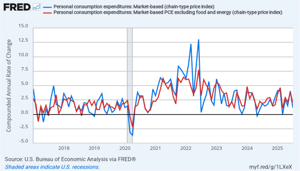
As usual, we need to note that Fed Chair Jerome Powell has frequently mentioned that inflation in non-market services can skew PCE inflation. Non-market services are services whose prices the BEA imputes rather than measures directly. For instance, the BEA assumes that prices of financial services—such as brokerage fees—vary with the prices of financial assets. So that if stock prices fall, the prices of financial services included in the PCE price index also fall. Powell has argued that these imputed prices “don’t really tell us much about … tightness in the economy. They don’t really reflect that.” The following figure shows 12-month headline inflation (the blue line) and 12-month core inflation (the red line) for market-based PCE. (The BEA explains the market-based PCE measure here.)
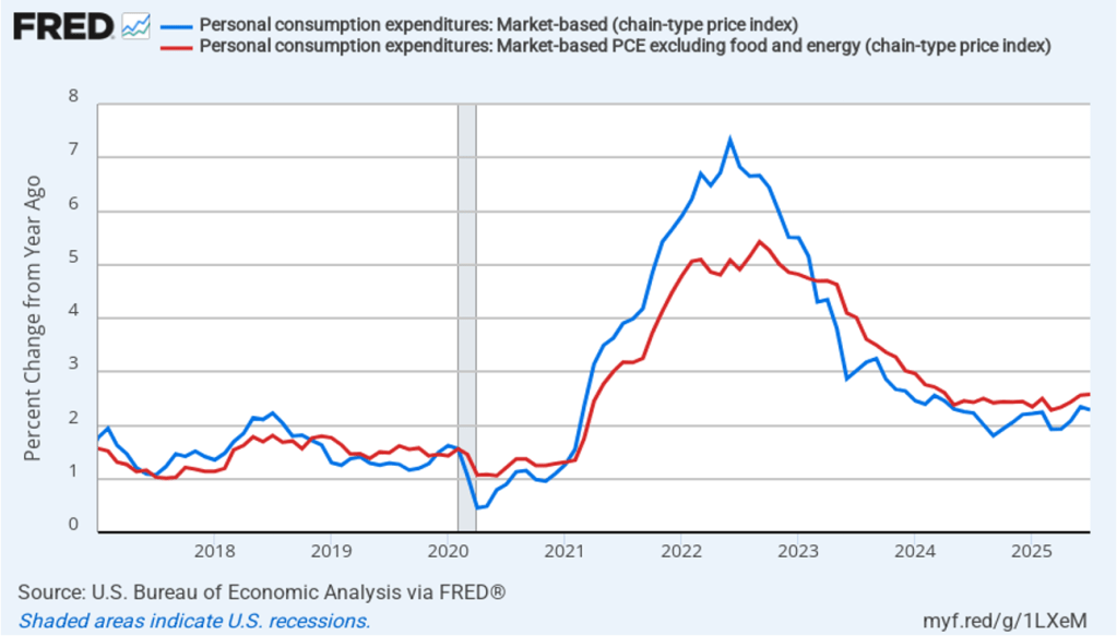
Headline market-based PCE inflation was 2.3 percent in July, unchanged from June. Core market-based PCE inflation was 2.6 percent in July, also unchanged from June. So, both market-based measures show inflation as stable but above the Fed’s 2 percent target.
In the following figure, we look at 1-month inflation using these measures. One-month headline market-based inflation declined sharply to 1.1 percent in July from 4.1 percent in June. One-month core market-based inflation also declined sharply to 2.1 percent in July from 3.8 percent in June. As the figure shows, the 1-month inflation rates are more volatile than the 12-month rates, which is why the Fed relies on the 12-month rates when gauging how close it is coming to hitting its target inflation rate. Still, looking at 1-month inflation gives us a better look at current trends in inflation, which these data indicate is slowing significantly.
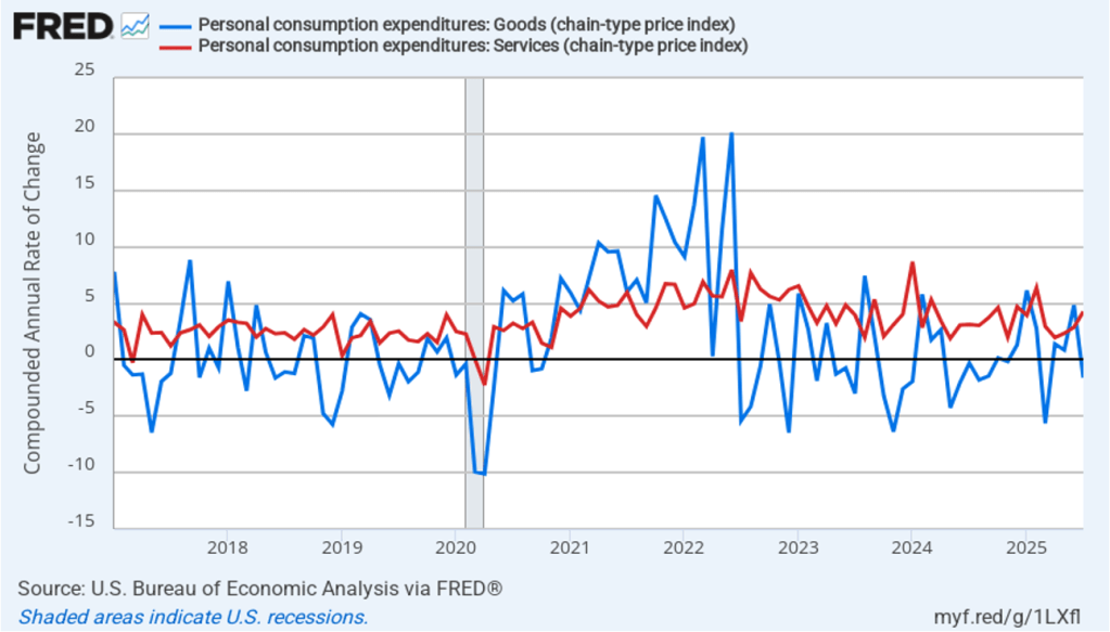
As we noted earlier, some of the increase in inflation is likely attributable to the effects of tariffs. The effect of tariffs are typically seen in goods prices, rather than in service prices because tariffs are levied primarily on imports of goods. As the following figure shows, one-month inflation in goods prices jumped in June to 4.8 percent, but then declined sharply to –1.6 in July. One-month inflation in services prices increased from 2.9 percent in June to 4.3 percent in July. Clearly, the 1-month inflation data—particularly for goods—are quite volatile.
Finally, these data had little effect on the expectations of investors trading federal funds rate futures. Investors assign an 86.4 percent probability to the Federal Open Market Committee (FOMC) cutting its target for the federal funds rate at its meeting on September 16–17 by 0.25 percentage point (25 basis points) from its current range of 4.25 percent to 4.5o percent. There has been some speculation in the business press that the FOMC might cut its target by 50 basis points at that meeting, but with inflation remaining above target, investors don’t foresee a larger cut in the target range happening.
Surprisingly Strong Jobs Report

Image created by ChatGTP=4o of workers on an automobile assembly line.
We noted in a blog post earlier this week that although the preliminary estimate from the Bureau of Economic Analysis (BEA) indicated that real GDP had declined during the first quarter of 2025, the report didn’t provide a clear indication that the U.S. economy was in recession. This morning (May 2), the Bureau of Labor Statistics (BLS) released its “Employment Situation” report (often called the “jobs report”) for April. The data in the report also show no sign that the U.S. economy is in a recession. Although there have been many stories in the media about businesspeople becoming increasingly pessimistic, we don’t yet see it in the employment data. We should add two caveats, however: 1. The effects of the large tariff increases the Trump Administration announced on April 2 are likely not reflected in the data from this report, and 2. at the beginning of a recession the data in the jobs report can be subject to large revisions.
The jobs report has two estimates of the change in employment during the month: one estimate from the establishment survey, often referred to as the payroll survey, and one from the household survey. As we discuss in Macroeconomics, Chapter 9, Section 9.1 (Economics, Chapter 19, Section 19.1), many economists and Federal Reserve policymakers believe that employment data from the establishment survey provide a more accurate indicator of the state of the labor market than do the household survey’s employment data and unemployment data. (The groups included in the employment estimates from the two surveys are somewhat different, as we discuss in this post.)
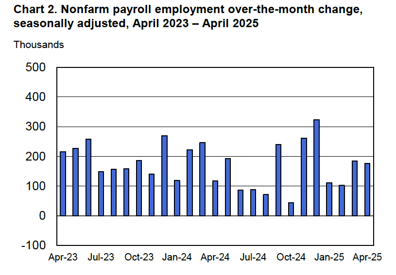
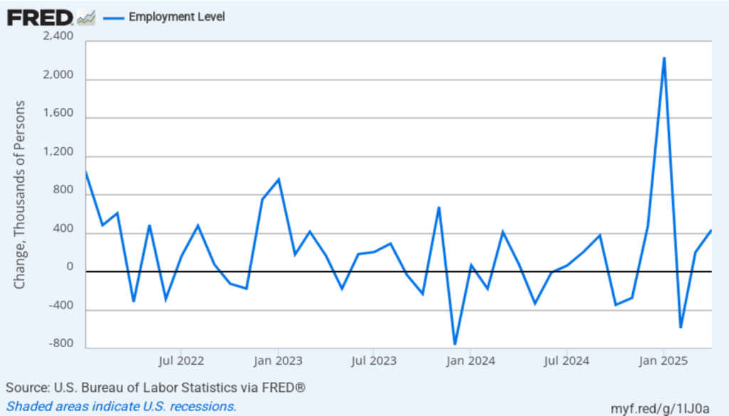
According to the establishment survey, there was a net increase of 177,000 jobs during April. This increase was well above the increase of 135,000 that economists surveyed had forecast. Somewhat offsetting this unexpectedly large increase was the BLS revising downward its previous estimates of employment in February and March by a combined 58,000 jobs. (The BLS notes that: “Monthly revisions result from additional reports received from businesses and government agencies since the last published estimates and from the recalculation of seasonal factors.”) The following figure from the jobs report shows the net change in payroll employment for each month in the last two years.
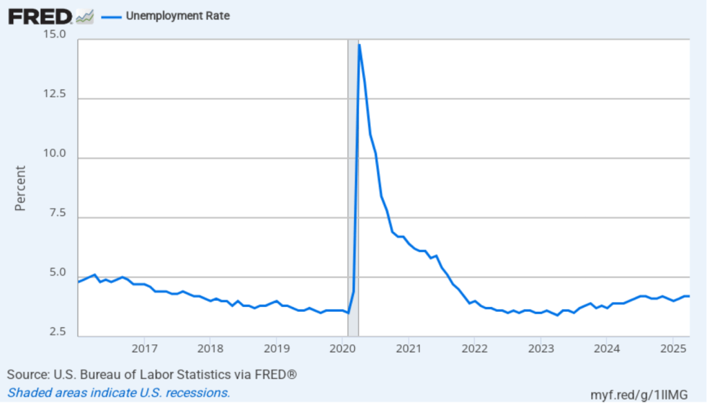
The unemployment rate was unchanged to 4.2 percent in April. As the following figure shows, the unemployment rate has been remarkably stable over the past year, staying between 4.0 percent and 4.2 percent in each month since May 2024. In March, the members of the Federal Open Market Committee (FOMC) forecast that the unemployment rate for 2025 would average 4.4 percent.
As the following figure shows, the monthly net change in jobs from the household survey moves much more erratically than does the net change in jobs from the establishment survey. As measured by the household survey, there was a net increase of 436,000 jobs in April, following an increase of 201,000 jobs in March. As an indication of the volatility in the employment changes in the household survey note the very large swings in net new jobs in January and February. In any particular month, the story told by the two surveys can be inconsistent with employment increasing in one survey while falling in the other. This month, however, both surveys showed net jobs increasing. (In this blog post, we discuss the differences between the employment estimates in the two surveys.)
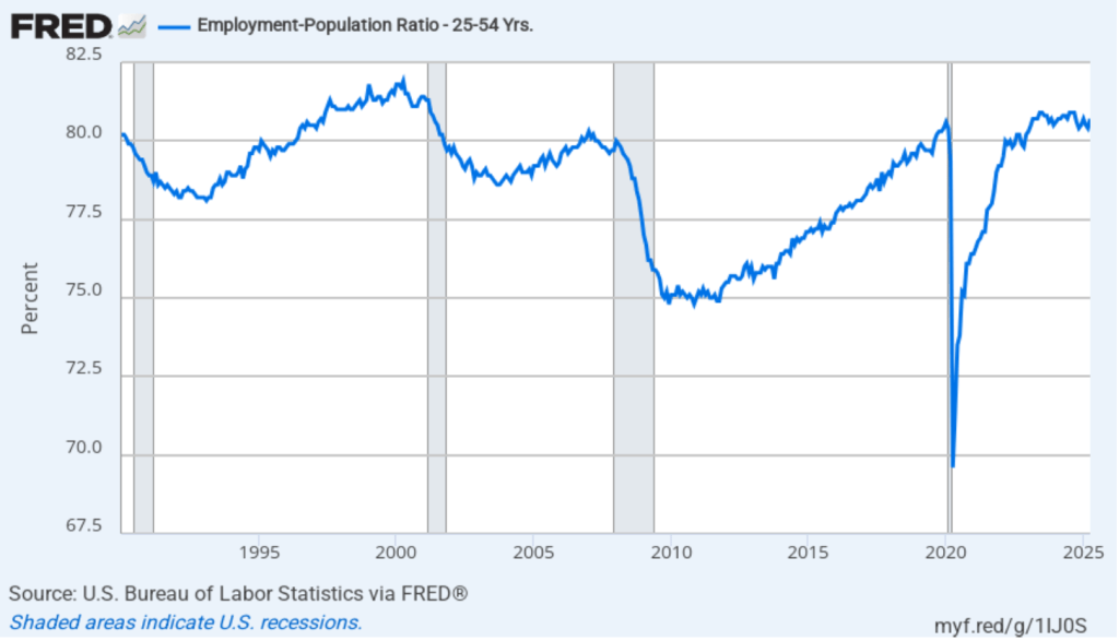
The household survey has another indication of continuing strength in the labor market. The employment-population ratio for prime age workers—those aged 25 to 54—increased from 80.4 percent in March to 80.7 percent in April. The prime-age employment-population ratio is somewhat below the high of 80.9 percent in mid-2024, but is above what the ratio was in any month during the period from January 2008 to January 2020.
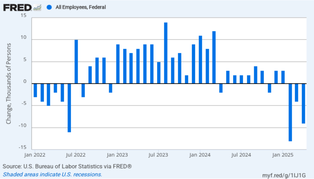
It remains unclear how many federal workers have been laid off since the Trump Administration took office. The establishment survey shows a decline in total federal government employment of 9,000 in April. However, the BLS notes that: “Employees on paid leave or receiving ongoing severance pay are counted as employed in the establishment survey.” It’s possible that as more federal employees end their period of receiving severance pay, future jobs reports may find a more significant decline in federal employment. To this point, the decline in federal employment has been too small to have a significant effect on the overall labor market.
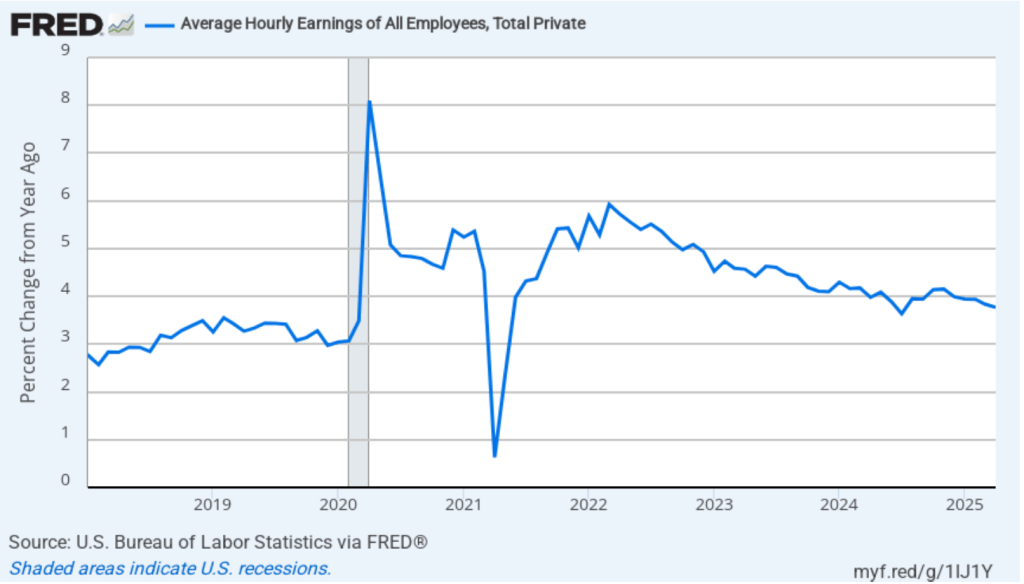
The establishment survey also includes data on average hourly earnings (AHE). As we noted in this post, many economists and policymakers believe the employment cost index (ECI) is a better measure of wage pressures in the economy than is the AHE. The AHE does have the important advantage of being available monthly, whereas the ECI is only available quarterly. The following figure shows the percentage change in the AHE from the same month in the previous year. The AHE increased 3.8 percent in April, which is unchanged from the March increase.
The following figure shows wage inflation calculated by compounding the current month’s rate over an entire year. (The figure above shows what is sometimes called 12-month wage inflation, whereas this figure shows 1-month wage inflation.) One-month wage inflation is much more volatile than 12-month wage inflation—note the very large swings in 1-month wage inflation in April and May 2020 during the business closures caused by the Covid pandemic. The April, the 1-month rate of wage inflation was 2.0 percent, down from 3.4 percent in March. If the 1-month increase in AHE is sustained, it would contribute to the Fed’s achieving its 2 percent target rate of price inflation.

Today’s jobs report leaves the situation facing the Federal Reserve’s policy-making Federal Open Market Committee (FOMC) largely unchanged. Looming over monetary policy, however, is the expected effect of the Trump Administration’s unexpectedly large tariff increases. As we note in this blog post, a large unexpected increase in tariffs results in an aggregate supply shock to the economy. In terms of the basic aggregate demand and aggregate supply model that we discuss in Macroeconomics, Chapter 13 (Economics, Chapter 23), an unexpected increase in tariffs shifts the short-run aggregate supply curve (SRAS) to the left, increasing the price level and reducing the level of real GDP.
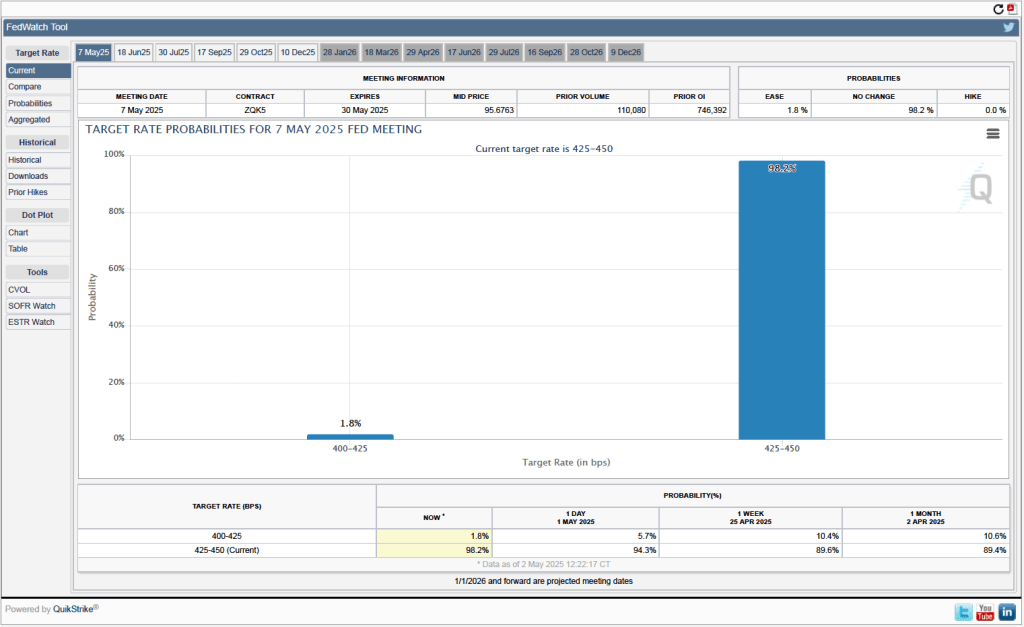
One indication of expectations of future changes in the target for the federal funds rate comes from investors who buy and sell federal funds futures contracts. (We discuss the futures market for federal funds in this blog post.) The data from the futures market indicate that, despite the potential effects of the surprisingly large tariff increases, investors don’t expect that the FOMC will cut its target for the federal funds rate at its May 6–7 meeting. As shown in the following figure, investors assign a 98.2 percent probability to the committee keeping its target unchanged at 4.25 percent to 4.50 percent at that meeting.
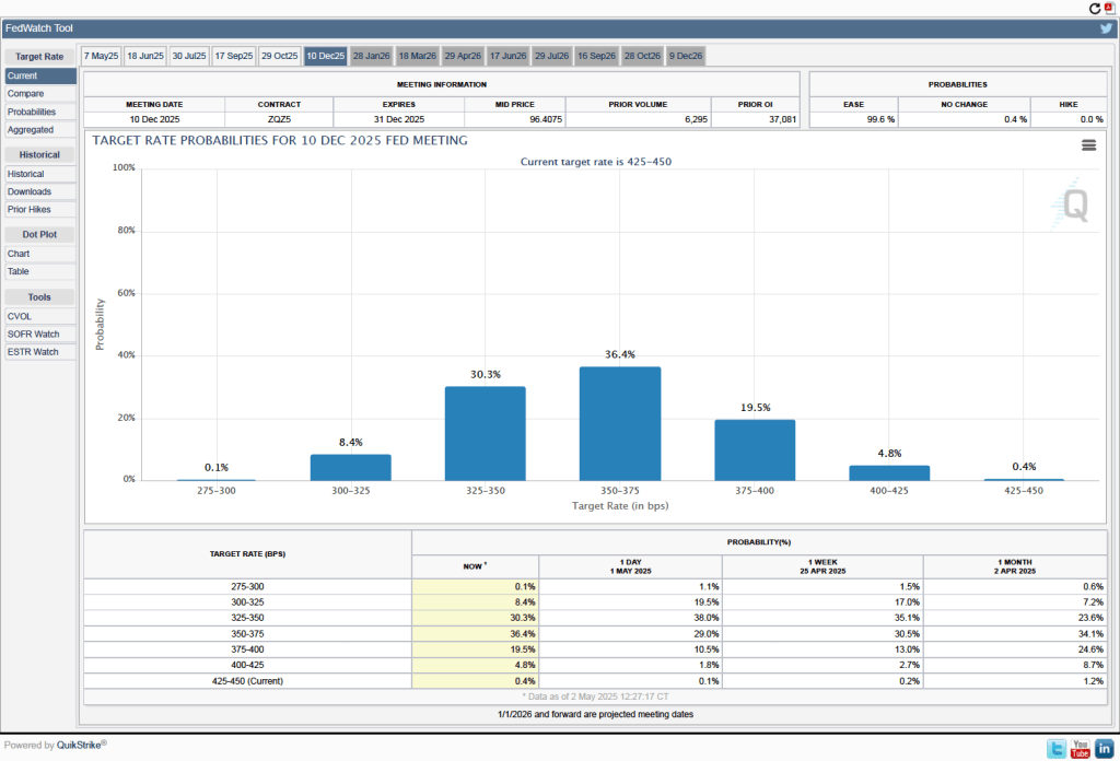
It’s a different story if we look at the end of the year. As the following figure shows, investors now expect that by the end of the FOMC’s meeting on December 9-10, the committee will have implemented at least three 0.25 percentage point (25 basis points) cuts in its target range for the federal funds rate. Investors assign a probability of 75.9 percent that the target range will end the year at 3.50 percent to 3.75 percent or lower. At their March meeting, FOMC members projected only two 25 basis point cuts this year—but that was before the announcement of the unexpectedly large tariff increases.
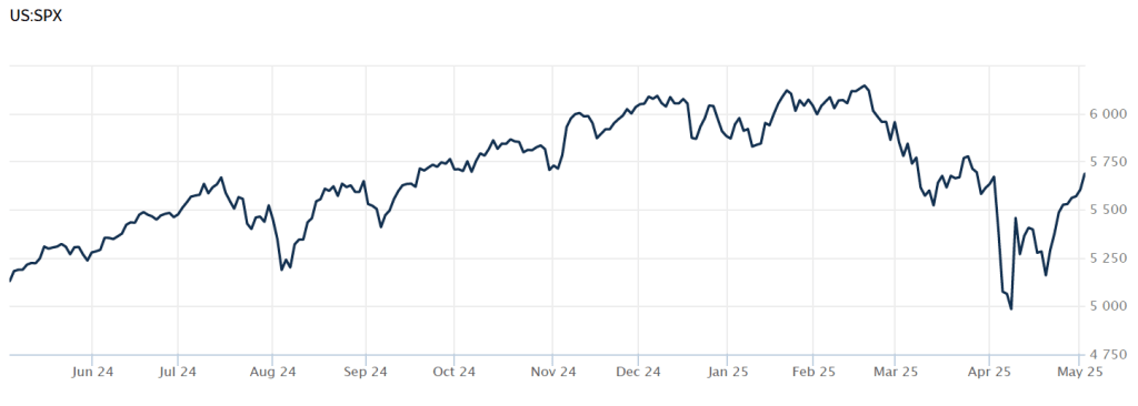
How the economy will fare for the remainder of the year depends heavily on what happens with respect to tariffs. News today that China and the United States may be negotiating lower tariff rates has contributed to rising stock prices. The following figure from the Wall Street Journal shows movements in the S&P stock index over the past year. The index declined sharply on April 2, following President Trump’s announcement of the tariff increases. As of 2 pm today, the S&P index has risen above its value on April 1, meaning that it has recovered all of the losses since the announcement of the tariff increases. The increase in stock prices likely indicates that investors expect that the tariff increases will end up being much smaller than those originally announced and that the chances of a recession happening soon are lower than they appeared to be on April 2.
Glenn Discusses Tariffs on Firing Line
Image created by ChatGTP-4o
Recently, Glenn appeared on the Firing Line program to discuss tariffs. Coincidentally, Margaret Hoover, the host of the program, is the great-granddaughter of Herbert Hoover. Herbert Hoover was the president who signed the Smoot-Hawley Tariff bill in 1930. We discussed the Smoot-Hawley Tariff in a recent blog post.
A Disagreement between Fed Chair Powell and Fed Governor Waller over Monetary Policy, and Can President Trump Replace Powell?

In this photo of a Federal Open Market Committee meeting, Fed Chair Jerome Powell is on the far left and Fed Governor Christopher Waller is the third person to Powell’s left. (Photo from federalreserve.gov)
This post discusses two developments this week that involve the Federal Reserve. First, we discuss the apparent disagreement between Fed Chair Jerome Powell and Fed Governor Christopher Waller over the best way to respond to the Trump Administration’s tariff increases. As we discuss in this blog post and in this podcast, in terms of the aggregate demand and aggregate supply model, a large unexpected increase in tariffs results in an aggregate supply shock to the economy, shifting the short-run aggregate supply curve (SRAS) to the left. The following is Figure 13.7 from Macroeconomics (Figure 23.7 from Economics) and illustrates the effects of an aggregate supply shock on short-run macroeconomic equilibrium.
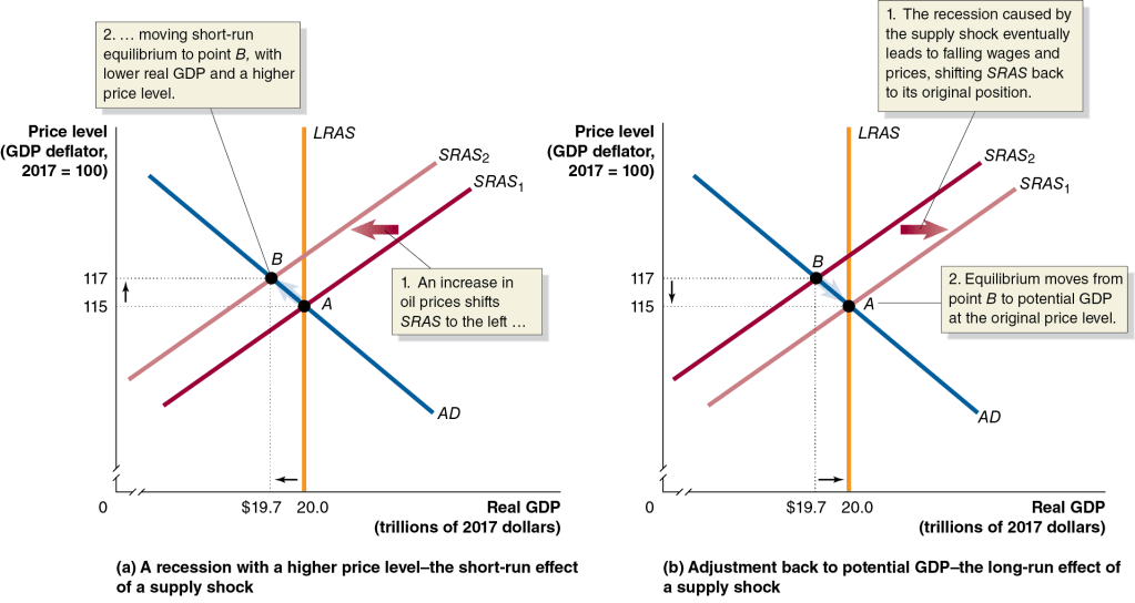
Although the figure shows the effects of an aggregate supply shock that results from an unexpected increase in oil prices, using this model, the result is the same for an aggregate supply shock caused by an unexpected increase in tariffs. Two-thirds of U.S. imports are raw materials, intermediate goods, or capital goods, all of which are used as inputs by U.S. firms. So, in both the case of an increase in oil prices and in the case of an increase in tariffs, the result of the supply shock is an increase in U.S. firms’ production costs. This increase in costs reduces the quantity of goods firms will supply at every price level, shifting the SRAS curve to the left, as shown in panel (a) of the figure. In the new macroeconomic equilibrium, point B in panel (a), the price level increases and the level of real GDP declines. The decline in real GDP will likely result in an increase in the unemployment rate.
An aggregate supply shock poses a policy dilemma for the Fed’s policymaking Federal Open Market Committee (FOMC). If the FOMC responds to the decline n real GDP and the increase in the unemployment rate with an expansionary monetary policy of lowering the target for the federal funds rate, the result is likely to be a further increase in the price level. Using a contractionary monetary policy of increasing the target for the federla funds rate to deal with the rising price level can cause real GDP to fall further, possibly pushing the economy into a recession. One way to avoid the policy dilemma from an aggregate supply shock caused by an increase in tariffs is for the FOMC to “look through”—that is, not respond—to the increase in tariffs. As panel (b) in the figure shows, if the FOMC looks through the tariff increase, the effect of the aggregate supply shock can be transitory as the economy absorbs the one-time increase in the price level. In time, real GDP will return to equilibrium at potential real GDP and the unemployment rate will fall back to the natural rate of unemployment.
On Monday (April 14), Fed Governor Christopher Waller in a speech to the Certified Financial Analysts Society of St. Louis made the argument for either looking through the macroeconomic effects of the tariff increase—even if the tariff increase turns out to be large, which at this time is unclear—or responding to the negative effects of the tariffs increases on real GDP and unemployment:
“I am saying that I expect that elevated inflation would be temporary, and ‘temporary’ is another word for ‘transitory.’ Despite the fact that the last surge of inflation beginning in 2021 lasted longer than I and other policymakers initially expected, my best judgment is that higher inflation from tariffs will be temporary…. While I expect the inflationary effects of higher tariffs to be temporary, their effects on output and employment could be longer-lasting and an important factor in determining the appropriate stance of monetary policy. If the slowdown is significant and even threatens a recession, then I would expect to favor cutting the FOMC’s policy rate sooner, and to a greater extent than I had previously thought.”
In a press conference after the last FOMC meeting on March 19, Fed Chair Jerome Powell took a similar position, arguing that: “If there’s an inflation that’s going to go away on its own, it’s not the correct response to tighten policy.” But in a speech yesterday (April 16) at the Economic Club of Chicago, Powell indicated that looking through the increase in the price level resulting from a tariff increase might be a mistake:
“The level of the tariff increases announced so far is significantly larger than anticipated. The same is likely to be true of the economic effects, which will include higher inflation and slower growth. Both survey- and market-based measures of near-term inflation expectations have moved up significantly, with survey participants pointing to tariffs…. Tariffs are highly likely to generate at least a temporary rise in inflation. The inflationary effects could also be more persistent…. Our obligation is to keep longer-term inflation expectations well anchored and to make certain that a one-time increase in the price level does not become an ongoing inflation problem.”
In a discussion following his speech, Powell argued that tariff increases may disrupt global supply chains for some U.S. industries, such as automobiles, in way that could be similar to the disruptions caused by the Covid pandemic of 2020. As a result: “When you think about supply disruptions, that is the kind of thing that can take time to resolve and it can lead what would’ve been a one-time inflation shock to be extended, perhaps more persistent.” Whereas Waller seemed to indicate that as a result of the tariff increases the FOMC might be led to cut its target for the federal funds sooner or to larger extent in order to meet the maximum employment part of its dual mandate, Powell seemed to indicate that the FOMC might keep its target unchanged longer in order to meet the price stability part of the dual mandate.
Powell’s speech caught the notice of President Donald Trump who has been pushing the FOMC to cut its target for the federal funds rate sooner. An article in the Wall Street Journal, quoted Trump as posting to social media that: “Powell’s termination cannot come fast enough!” Powell’s term as Fed chair is scheduled to end in May 2026. Does Trump have the legal authority to replace Powell earlier than that? As we discuss in Macroeconomics, Chapter 27 (Economics Chapter 17), according to the Federal Reserve Act, once a Fed chair is notimated to a four-year term by the president (President Trump first nominated Powell to be chair in 2017 and Powell took office in 2018) and confirmed by the Senate, the president cannot remove the Fed chair except “for cause.” Most legal scholars argue that a president cannot remove a Fed chair due to a disagreement over monetary policy.
Article I, Section II of the Constitution of the United States states that: “The executive Power shall be vested in a President of the United States of America.” The ability of Congress to limit the president’s power to appoint and remove heads of commissions, agencies, and other bodies in the executive branch of government—such as the Federal Reserve—is not clearly specified in the Constitution. In 1935, a unanimous Supreme Court ruled in the case of Humphrey’s Executor v. United States that President Franklin Roosevelt couldn’t remove a member of the Federal Trade Commission (FTC) because in creating the FTC, Congress specified that members could only be removed for cause. Legal scholars have presumed that the ruling in this case would also bar attempts by a president to remove members of the Fed’s Board of Governors because of a disagreement over monetary policy.
The Trump Administration recently fired a member of the National Labor Relations Board and a member of the Merit Systems Protection Board. The members sued and the Supreme Court is considering the case. The Trump Adminstration is asking the Court to overturn the Humphrey’s Executor decision as having been wrongly decided because the decision infringed on the executive power given to the president by the Constitution. If the Court agrees with the administration and overturns the precdent established by Humphrey’s Executor, would President Trump be free to fire Chair Powell before Powell’s term ends? (An overview of the issues involved in this Court case can be found in this article from the Associated Press.)
The answer isn’t clear because, as we’ve noted in Macroeconomics, Chapter 14, Section 14.4, Congress gave the Fed an unusual hybrid public-private structure and the ability to fund its own operations without needing appropriations from Congress. It’s possible that the Court would rule that in overturning Humphrey’s Executor—if the Court should decide to do that—it wasn’t authorizing the president to replace the Fed chair at will. In response to a question following his speech yesterday, Powell seemed to indicate that the Fed’s unique structure might shield it from the effects of the Court’s decision.
If the Court were to overturn its ruling in Humphrey’s Executor and indicate that the ruling did authorize the president to remove the Fed chair, the Fed’s ability to conduce monetary policy independently of the president would be seriously undermined. In Macroeconomics, Chapter 17, Section 17.4 we review the arguments for and against Fed independence. It’s unclear at this point when the Court might rule on the case.
The U.S.-China Trade War Illustrated in Two Graphs from the Peterson Institute
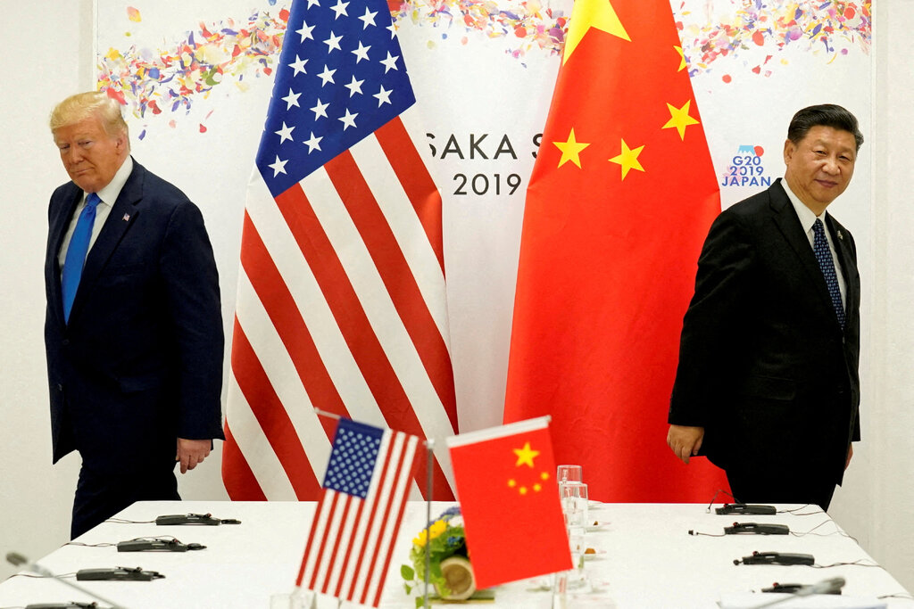
Photo of U.S. President Donald Trump and China President Xi Jinping from Reuters.
The tit-for-tat tariff increases the U.S. and Chinese governments have levied on each other’s imports have reached dizzying heights today (April 11). The United States has imposed a tariff rate of 134.7 percent on imports from China, while China has imposed a tariff rate of 147.6 percent on imports from the United States. On all other countries—the rest of the world (ROW)—the United States imposes an average tariff rate of 10.5 percent, which is a sharp increase reflecting the Trump Administration’s imposition of a tariff of at least 10 percent on all countries. The government of China imposes a tariff rate of 6.5 percent on the ROW.
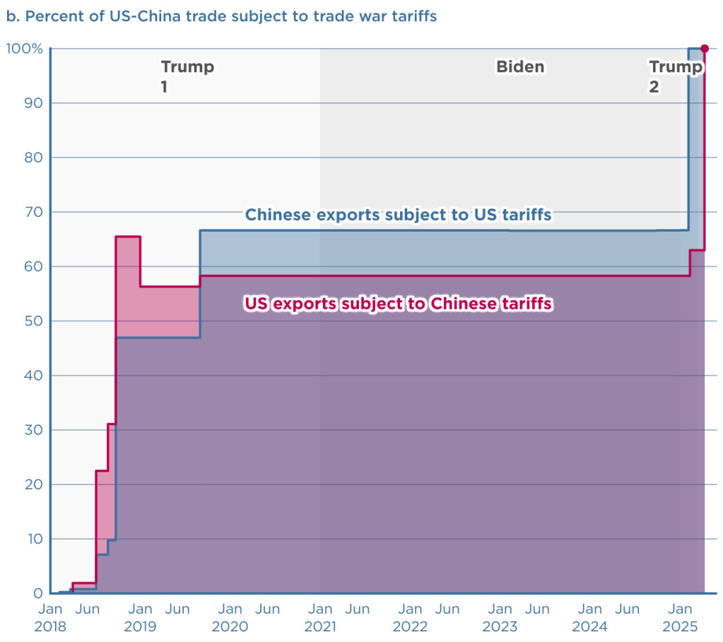
The Peterson Institute for International Economics (PIIE) is a think tank located in Washington, DC. Chad Brown, a senior fellow at PIIE, has created two charts that dramatically illustrate the current state of the U.S.-China trade war. The first chart shows the changes since the beginning of the first Trump Administration in 2017 in the tariff rates the countries have imposed on each other’s imports.

The second chart shows the percentage of each country’s exports to the other country that have been subject to tariffs. As of today, 100 percent of each country’s exports are subject to the other country’s tariffs.
Finally, we repeat a figure from an earlier blog post showing changes over time in the average tariff rate the United States levies on imports. The value for 2025 of 16.5 percent is an estimate by the Tax Foundation and assumes that the tariff rates that the Trump Administration announced on April 2 go into force, although the rates are currently suspended for 90 days—apart from those imposed on China. (An average tariff rate of 16.5 percent would be the highest levied by the United States since 1937.)

Thanks to Fernando Quijano for preparing this figure.
CPI Inflation Slows More than Expected
Image generated by Chat-GTP-4o
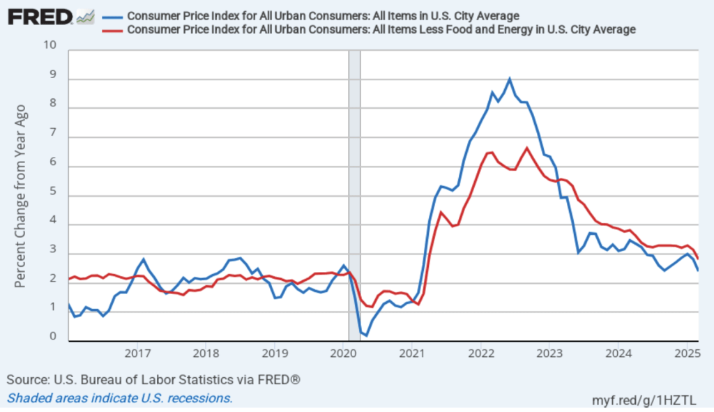
Today (April 10), the Bureau of Labor Statistics (BLS) released its monthly report on the consumer price index (CPI). The following figure compares headline inflation (the blue line) and core inflation (the red line).
- The headline inflation rate, which is measured by the percentage change in the CPI from the same month in the previous year, was 2.4 percent in March—down from 2.8 percent in February.
- The core inflation rate, which excludes the prices of food and energy, was 2.8 percent in March—down from 3.1 percent in February.
Both headline inflation and core inflation were below what economists surveyed had expected.
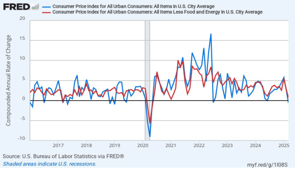
In the following figure, we look at the 1-month inflation rate for headline and core inflation—that is the annual inflation rate calculated by compounding the current month’s rate over an entire year. Calculated as the 1-month inflation rate, headline inflation (the blue line) fell sharply from 2.6 percent in March to –0.6 percent—that is, the economy experienced deflation in March. Core inflation (the red line) decreased from 2.6 percent in February to 0.7 percent in March.
Overall, considering 1-month and 12-month inflation together, inflation slowed significantly in March. Of course, it’s important not to overinterpret the data from a single month. The figure shows that 1-month inflation rate is particularly volatile. Also note that the Fed uses the personal consumption expenditures (PCE) price index, rather than the CPI, to evaluate whether it is hitting its 2 percent annual inflation target.
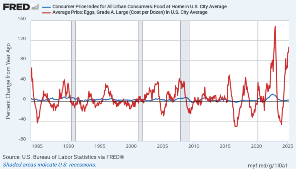
There’s been considerable discussion in the media about continuing inflation in grocery prices. In the following figure the blue line shows inflation in the CPI category “food at home,” which is primarily grocery prices. Inflation in grocery prices was 2.4 percent in March, up from 1.8 percent in February, but still far below the peak of 13.6 percen in August 2022. Although, on average, grocery price inflation has been low over the past 18 months, there have been substantial increases in the prices of some food items. For instance, egg prices—shown by the red line—increased by 108.1 percent in March. But, as the figure shows, egg prices are usually quite volatile month-to-month, even when the country is not dealing with an epidemic of bird flu.
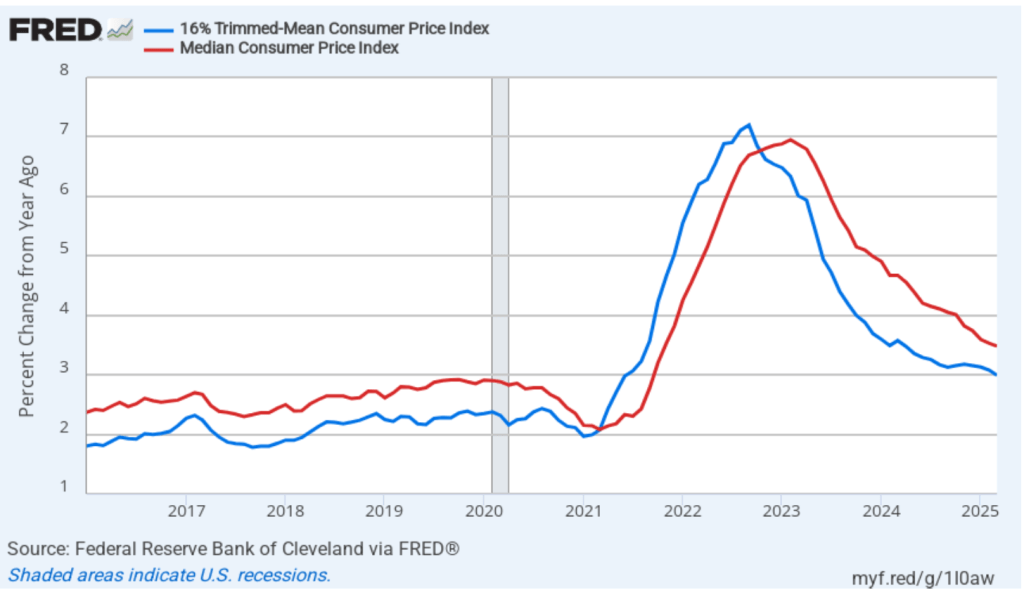
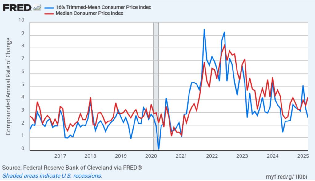
To better estimate the underlying trend in inflation, some economists look at median inflation and trimmed mean inflation.
- Median inflation is calculated by economists at the Federal Reserve Bank of Cleveland and Ohio State University. If we listed the inflation rate in each individual good or service in the CPI, median inflation is the inflation rate of the good or service that is in the middle of the list—that is, the inflation rate in the price of the good or service that has an equal number of higher and lower inflation rates.
- Trimmed-mean inflation drops the 8 percent of goods and services with the highest inflation rates and the 8 percent of goods and services with the lowest inflation rates.
The following figure shows that 12-month trimmed-mean inflation (the blue line) was 3.0 percent in March, down from 3.1 percent in February. Twelve-month median inflation (the red line) also declined slightly from 3.1 percent in February to 3.0 percent in March.
The following figure shows 1-month trimmed-mean and median inflation. One-month trimmed-mean inflation fell from 3.3 percent in February to 2.6. percent in March. One-month median inflation increased from 3.5 percent in February to 4.1 percent in March. These data are noticeably higher than either the 12-month measures for these variables or the 1-month and 12-month measures of headline and core inflation. Again, though, all 1-month inflation measures can be volatile.
There isn’t much sign in today’s CPI report that the tariffs recently imposed by the Trump Administration have affected retail prices. President Trump announced yesterday that many of the tariffs would be suspended for at least 90 days, although the across-the-board tariff of 10 percent remains in place and a tariff of 145 percent has been imposed on goods imported from China. It would surprising if those tariff increases don’t begin to have at least some effect on the CPI over the next few months. As we noted in this post from earlier in the month, Tariffs pose a dilemma for the Fed, because tariffs have the effect of both increasing the price level and reducing real GDP and employment.
What are the implications of this CPI report for the actions the Federal Reserve’s policymaking Federal Open Market Committee (FOMC) may take at its next two meetings? Investors who buy and sell federal funds futures contracts still do not expect that the FOMC will cut its target for the federal funds rate at its next two meetings. (We discuss the futures market for federal funds in this blog post.) Today, investors assigned only a 29.9 percent probability that the Fed’s policymaking Federal Open Market Committee (FOMC) will cut its target from the current 4.25 percent to 4.50 percent range at its meeting on May 6–7. Investors assigned a probability of 85.2 percent that the FOMC would cut its target after its meeting on June 17–18 by at least 0.25 percent (or 25 basis points).
By the time the FOMC meets again in early May we may have more data on the effects the tariffs are having on the economy.
What Happened after Smoot-Hawley?
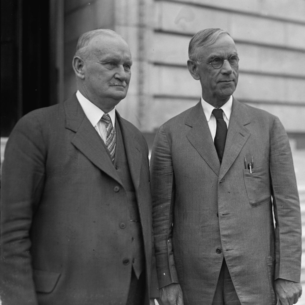
Congressman Willis Hawley of Oregon and Senator Reed Smoot of Utah (Photo from the U.S. Library of Congress via the Wall Street Journal)
Until last week, the most famous example of the United States dramatically increasing tariffs on foreign imports was the Smoot-Hawley Tariff, which was passed by Congress and signed into law by President Herbet Hoover in June 1930. The website of the U.S. Senate describes the bill as “among the most catastrophic acts in congressional history.”
Did the Smoot-Hawley Tariff cause the Great Depression? According to the National Bureau of Economic Research’s business cycle dates, the Great Depression began in August 1929, well before the passage of Smoot-Hawley. By June 1930, industrial production had already declined in the United States by more than 17 percent. So, even if the downturn had ended at that point it would still have been severe. The contraction phase of the Depression continued until March 1933, by which time industrial production had declined more than 51 percent. That was the largest decline in U.S. history
If Smoot-Hawley didn’t cause the Depression, did it contribute to the Depression’s length and severity? Most economists believe that it did by contributing to the collapse of the global trading system, thereby reducing U.S. exports, aggregate demand, and production and employment.
Some years ago, Tony wrote an overview of Smoot-Hawley that discusses its causes and effects in more detail. A key question in assessing the effects of Smoot-Hawley is the extent to which key trading partners of the United States raised their tariffs in retaliation. The clearest case is Canada, which in 1930 was the leading trading partner of the United States. Canadian Prime Minister William Lyon Mackenzie King and the Liberal Party significantly raised tariffs on U.S. imports in explicit retaliation for Smoot-Hawley. This journal article that Tony co-wrote with two Lehigh colleagues discusses the empirical evidence for this conclusion. (The link takes you to the Jstor site. You may be able to read or download the whole article by clicking on the link on that page and entering the name of your college or university.)
The Trump Administration seems to be attempting a major reordering of the global trading system. A Canadian prime minister in the 1930s tried something similar. Richard Bedford Bennett became prime minister after his Conservative Party defeated Mackenzie King’s Liberal Party in the 1935 Canadian election. Bennett hoped to replace the U.S. market with the markets in England and other countries in the British Commonwealth. He argued that, taken together, the Commonwealth countries had sufficient resources to be largely self-sufficient and need not rely on trade with non-Commonwealth countries. In the end, Bennett was unsuccessful for reasons that Tony and a Lehigh colleague explore in this journal article.
