Supports: Chapter 2, Trade-offs, Comparative Advantage, and the Market System [Econ, Micro, Macro, and Essentials]; Chapter 9, Comparative Advantage and the Gains from International Trade [Econ and Micro; Macro Chapter 7; and Essentials Chapter 19]; Chapter 22, Aggregate Expenditure and Output in the Short Run [Macro Chapter 12].
WILL APPLE START MAKING IPHONES IN THE UNITED STATES?
Apple, like many U.S. firms, relies on a global supply chain (sometimes also called a global value chain) comprised of firms in dozens of countries to make the components used in Apple’s products. (See Hubbard/O’Brien Chapter 2, Section 2.3 of Hubbard and O’Brien Economics and Microeconomics). This strategy has allowed Apple to take advantage of both lower production costs and the engineering and manufacturing skills of firms in other countries to produce iPhones, iPads, iWatches, and MacBooks. But during the coronavirus pandemic, Apple found its supply chain disrupted because many of its suppliers located in China were forced to close for several months.
Because of the coronavirus pandemic and the trade war between the United States and China, many U.S. firms, including Apple, were considering moving some of their operations out of China. (The trade war is discussed in Chapter 9, section 9.5 of Hubbard and O’Brien Economics and Microeconomics, Chapter 7, Section 7.5 of Macroeconomics.) As an article on bloomberg.com put it, these firms were “actively seeking ways to diversify their supply chains and reduce their dependence on any single country, no matter how attractive.” For example, two Taiwanese firms, Wistron and Pegatron, which had used factories in China to assemble iPhones were moving some factories to India, Vietnam, and Taiwan.
It seemed unlikely, though, that production of iPhones would move back to the United States. Why not? First, manufacturing employment has been in decline in the United States since long before U.S. firms began using suppliers based in China. In 1947, shortly after the end of World War II, 33 percent of U.S. workers were employed in manufacturing. By 2001, when China became a member of the World Trade Organization, that percentage had already declined to 12 percent. In 2019, it was 9 percent.
Manufacturing production in the United States has held up better than manufacturing employment. The Federal Reserve’s index of manufacturing production increased more than 250 percent between the beginning of 1972 and the beginning of 2020. U.S. manufacturing has been able to increase output while employment has declined because of increases in productivity. The increases in productivity have relied, in part, on increased use of robotics, particularly in assembly line work, such as the production of automobiles. The United States has a comparative advantage in producing goods and services that require skilled labor and involve artificial intelligence, machine learning, and the use of other sophisticated computer programing. Manufacturing that relies on lower-skilled labor, such as textile and shoe production, has been mostly moved overseas.
The Taiwanese firms Foxconn, Wistron, and Pegatron assemble iPhones, primarily in factories in China and elsewhere in Asia where large quantities of unskilled labor are available. Some components of the iPhone that require skilled labor and sophisticated engineering, including the screens, the touchscreen controller, and the Wi-Fi chip, are produced by U.S. firms and shipped to China for final assembly. In fact, surprisingly, the value of the U.S.-made components exceeds the value of assembling the iPhone in Chinese factories. (See Hubbard and O’Brien Economics, Chapter 22, Section 22.3 and Macroeconomics, Chapter 12, Section 12.3).
Factory assembly lines, like those in China making iPhones, need to be flexible to respond quickly to Apple introducing new models. So, in addition, to hundreds of thousands of unskilled workers in its assembly plants, Foxconn and other firms operating in China hire thousands of engineers. Typically, these engineers do not have college degrees, but they have sufficient training to rapidly redesign and reconfigure assembly lines to produce new models. In 2010, when President Barack Obama pressed Steve Jobs, the late Apple CEO, to produce iPhones in the United States, Jobs pointed to lack of sufficient workers with engineering skills to make such production possible. Jobs stated that he would need 30,000 such engineers if Apple were to make iPhones in the United States, but “You can’t find that many in America to hire.”
The situation hasn’t changed much in the past 10 years. As an article in the Wall Street Journal observed in March 2020, in addition to a large number of unskilled workers, Foxconn employs in China, “Tens of thousands of experienced manufacturing engineers [to] oversee the [production] process. Finding a comparable amount of unskilled and skilled labor [elsewhere] is impossible.”
Although some firms were attempting to reduce their reliance on Chinese factories in response to the coronavirus pandemic, because the United States lacks a comparative advantage in the assembly of consumer electronics, it seemed unlikely that those factories would be relocated here. But the coronavirus pandemic may lead some U.S. firms to change their supply chains in other ways. For instance, firms may now put greater value on redundancy. Apple might underwrite the cost to its suppliers of building facilities in several Asian countries to assemble iPhones. In the event of problems occurring in one country, this redundant capacity would allow production to switch from factories in one country to factories in other countries.
Similarly, some firms may rethink their inventory management. Before the 1970s, most manufacturing firms kept substantial inventories of parts and components. Retail firms often kept substantial inventories of goods in warehouses. This approach began to change during the 1970s, as Toyota pioneered just-in-time inventory systems in which firms accept shipments from suppliers as close as possible to the time they will be needed. Most manufacturers in the United States and elsewhere adopted these systems, as did many retailers.
For example, at Walmart, as goods are sold in the stores, this point-of-sale information is sent electronically to the firm’s distribution centers to help managers determine what products to ship to each store. This distribution system allows Walmart to minimize its inventory holdings. Because Walmart sells 15 to 25 percent of all the toothpaste, disposable diapers, dog food, and other products sold in the United States, it has involved many manufacturers in its supply chain. For example, a company such as Procter & Gamble, one of the world’s largest manufacturers of toothpaste, laundry detergent, and toilet paper, receives Wal-Mart’s point-of-sale and inventory information electronically. Procter & Gamble uses that information to determine its production schedules and the quantities and timing of its shipments to Walmart’s distribution centers.
But as the pandemic disrupted supply chains, many manufacturers had to suspend production because they did not receive timely shipments of parts. Similarly, Walmart and other retailers experienced stockouts—sales lost because the goods consumer want to buy aren’t on the shelves.
In 2020, firms were reconsidering their supply chains as they evaluated whether to underwrite the building of redundant capacity among their suppliers and whether to reduce the extent to which they relied on just-in-time inventory systems.
Sources: Debby Wu, “Not Made in China Is Global Tech’s Next Big Trend,” bloomberg.com, March 31, 2020; Yossi Sheffi, “Commentary: Supply-Chain Risks From the Coronavirus Demand Immediate Action,” Wall Street Journal, February 18, 2020; Tripp Mickle and Yoko Kubota, “Tim Cook and Apple Bet Everything on China. Then Coronavirus Hit,” Wall Street, March 3, 2020; and Walter Isaacson, Steve Jobs, New York: Simon & Schuster, 2011, pp. 544-547.
Question: Suppose that you’re a manager at Apple. Given the coronavirus pandemic, Apple is considering whether to underwrite the cost to its suppliers, such as Foxconn, of building redundant factories in countries outside of China.. The goal is to reduce the production problems that occur when factories are concentrated in a single country during a pandemic or other disaster. Your manager asks you to prepare a brief evaluation of this idea. What factors should you take into account in your evaluation?
During the initial UNWRITTEN webinar from Pearson, Glenn Hubbard had a conversation with Jaylen Brown, a Pearson Campus Ambassador as well as a student at University of Central Florida -also Glenn’s undergrad alma mater!
Over the 30-minute broadcast, they discussed topics of relevance to all students – real world outlook on jobs, supply and demand, and the policies aimed at relief. Glenn talks of recovery shaped like a Nike swoosh with a sharp decline and a slightly longer climb back to normalcy. Check out the full episode now posted on YouTube!
On April 10th Glenn Hubbard and Tony O’Brien sat down together to discuss some of the larger impacts of the pandemic.
In these 18 minutes, Glenn and Tony discuss the fiscal & monetary response, the future relationship of the US Treasury and the Federal Reserve System, as well as several other topics.
Economics – Chapter 7, The Economics of Health Care; Chapter 18, GDP: Measuring Total Production and Income; Micro – Chapter 7, The Economics of Health Care; Macro Chapter 5, The Economics of Health Care; Chapter 8, GDP: Measuring Total Production and Income; Essentials – Chapter 5, The Economics of Health Care; Chapter 12, GDP: Measuring Total Production and Income
Lessons from the Influenza Pandemic of 1918-1919 for the Coronavirus Pandemic of 2020
The coronavirus pandemic of 2020 was by far the most serious epidemic to affect the United States since the influenza pandemic of 1918-1919, sometimes called the Spanish Flu. Does the 1918-1919 influenza pandemic provide clues that help us predict how the coronavirus pandemic might affect the U.S. economy? In this discussion, we:
Summarize scholarly and popular articles that address this question.
Provide links to the full articles.
Draw some tentative conclusions.
SCHOLARLY ARTICLES
What Effect Did the 1918-1919 Influenza Pandemic Have on Death Rates and Real GDP?
A National Bureau of Economic Research (NBER) Working Paper by Robert Barro of Harvard University, José Ursúa of Dodge & Cox, a mutual fund firm, and Joanna Weng of EverLife, an online food firm, estimate that the 1918-1919 pandemic killed about 39 million or about 2.0 percent of the world’s population. An equivalent percentage of the world’s population today would be 150 million people. The pandemic killed about 550,000 people in the United States or about 0.5 percent of the population. If the death rate in the United States from the coronavirus were also 0.5 percent, the result would be 1.65 million deaths.
Barro, Ursúa, and Weng also estimate that the influenza pandemic reduced real GDP per capita in the typical country by 6 percent and real private consumption per capita by 8 percent. The comparable estimates for the United States are a decline in real GDP per capita of 1.5 percent and of real private consumption per capita by 2.0 percent. They conclude that, “At this point, the probability that COVID-19 reaches anything close to the Great Influenza Pandemic seems remote, given advances in public-health care and measures that are being taken to mitigate propagation.” The following table summarizes the Barro, Ursúa, and Weng estimates.
The What Effect Did Air Pollution Have on theWhat Effect Did Social Distancing Have on the 1918-1919 Influenza Pandemic?
A working paper by Sergio Correia, of the Federal Reserve Board, Stephan Luck of the Federal Reserve Bank of New York, and Emil Verner of the MIT School of Management examines the benefits and costs of non-pharmaceutical interventions (NPIs)—such as social distancing policies—during the 1918 pandemic. They find that cities that implemented NPIs early and maintained them for longer experienced both lower mortality and higher economic growth, as measured by increases in manufacturing employment between 1914 and 1919. The cities of Seattle, Portland, Oakland, Los Angeles, and Omaha particularly stand out in this respect. Cities such as Pittsburgh, Philadelphia, and Boston that were slow to implement NPIs, or kept them in place for shorter periods, experienced both higher mortality rates and slower economic growth. The authors note: “This suggests that NPIs play a role in attenuating mortality, but without reducing economic activity. If anything, cities with longer NPIs grow faster in the medium term.”
Correia, Luck, and Verner find substantial positive economic effect from early and prolonged implementation of NPIs: “Reacting 10 days earlier to the arrival of the pandemic in a given city increases manufacturing employment by around 5% in the post period. Likewise, implementing NPIs for an additional 50 days increases manufacturing employment by 6.5% after the pandemic.” They suggest that early implementation of NPIs may “flatten the curve,” keeping hospitals from being overwhelmed, and reducing mortality. They note that aggressive early use of NPIs appear to have successfully reduced both mortality rates and economic losses in Taiwan and Singapore.
What Effect Did Air Pollution Have on the 1918-1919 Influenza Pandemic?
Karen Clay and Edson Severnini of Carnegie Mellon University and Joshua Lewis of the Université de Montréal find that U.S. cities with worse air pollution—largely as the result of local utilities using more coal to generate electric power—suffered significantly higher death rates: “Cities that used more coal experienced tens of thousands of excess deaths in 1918 relative to cities that used less coal with similar pre-pandemic socioeconomic conditions and baseline health.”
Sources: Robert J. Barro, José F. Ursúa, and Joanna Weng, “The Coronavirus and the Great Influenza Pandemic: Lessons from the “Spanish Flu” for the Coronavirus’s Potential Effects on Mortality and Economic Activity,” National Bureau of Economic Research, March 2020—The paper can be found here (the NBER is providing free access to working papers related to the coronavirus epidemic): https://www.nber.org/papers/w26866.pdf; Sergio Correia, Stephan Luck, and Emil Verner, “Pandemics Depress the Economy, Public Health Interventions Do Not: Evidence from the 1918 Flu,” March 26, 2020—the paper can be found here: ; and Karen Clay, Joshua Lewis, and Edson Severnini, “Pollution, Infectious Disease, and Mortality: Evidence from the 1918 Spanish Influenza Pandemic,” Journal of Economic History, Vol. 78, No. 4, December 2018, pp. 1179-1209—The NBER working paper version can be found here.
Did People Who Were in Utero during the 1918-1919 Influenza Pandemic Suffer Negative Health Effects?
In an influential academic article published in 2008, Douglas Almond of Columbia University argued that people who were in utero during the influenza pandemic “displayed reduced educational attainment, increased rates of physical disability, lower income, lower socioeconomic status, and higher transfer payments compared with other birth cohorts.” However, research by Ryan Brown of the University of Colorado, Denver and Duncan Thomas of Duke University provides evidence that the women who became pregnant during the pandemic were likely to be from lower socio-economic status than were women who became pregnant during earlier or later years. This result is attributable to the pandemic occurring during 1918 when many men of higher-than-average socio-economic status had been drafted to fight in World War I. After correcting for the socio-economic status of the parents of people who were in utero during the pandemic, Brown and Thomas find that “there is little evidence that individuals born in 1919 have worse socio-economic outcomes in adulthood relative to surrounding birth cohorts.”
Brian Beach of the College of William and Mary, Joseph P. Ferrie of Northwestern University, and Martin H. Saavedra of Oberlin College study this issue using individual data from the population censuses of 1920 and 1930 linked to World War II enlistment records. Their sample is large enough to contain many brothers, which allows them to completely control for the effects of socio-economic factors. They conclude that in utero exposure reduced high school graduation rates by about 2 percentage points but had no effect on adult height, weight, or body mass index (BMI).
Sources: Douglas Almond, “Is the 1918 Influenza Pandemic Over? Long- Term Effects of In Utero Influenza Exposure in the Post-1940 U.S. Population,” Journal of Political Economy, Vol. 114, No. 4, August 2006, pp. 672-712; Ryan Brown and Duncan Thomas, “On the Long Term Effects of the 1918 U.S. Influenza Pandemic,” June 2018 (https://clas.ucdenver.edu/ryan-brown/sites/default/files/attached-files/brownthomas_0.pdf); and Brian Beach, Joseph P. Ferrie, and Martin H. Saavedra, “Fetal Shock or Selection? The 1918 Influenza Pandemic and Human Capital Development,” National Bureau of Economic Research, Working Paper 24725, June 2018 (https://www.nber.org/papers/w24725).
POPULAR ARTICLES
An article on msnbc.com notes that compared with the 1918-1919 influenza pandemic, the coronavirus pandemic may turn out to be more contagious but with a lower death rate (although the death rate from the coronavirus appeared higher when the article was first published).
In an opinion column in the New York Times, John Barry, a professor of public health at Tulane University and the author of the best-known history of the 1918-1919 pandemic, notes that an analysis of differences in the policies enacted among U.S. cities during the influenza pandemic indicates that when social distancing happened “before a virus spreads throughout the community, [it] did flatten the curve”—that is, it avoided a spike in deaths that would overwhelm hospitals.
An article on nationalgeographic.com has some interesting graphs showing death rates from the influenza pandemic across many U.S. cities. Some cities experienced two peaks during 1918, while others did not. The article, which summarizes earlier epidemiological research, concludes that “death rates were around 50 percent lower in cities that implemented preventative measures early on, versus those that did so late or not at all.” The cities that kept these measures in place longest were the ones that did not experience a second spike in death rates.
Although the nationalgeographic.com article attributes the relatively low death rate in New York City during the influenza pandemic to the early implementation of quarantine and other public health measures, this op-ed in the New York Timesby historian Mike Wallace indicates that the city did not close its public schools or most of its theaters, although it did levy fines to enforce a prohibition on public spitting—a common habit among men at the time.
This essay in the Wall Street Journal by a medical doctor and adjunct professor at the Duke Global Health Institute reviews the course of the influenza pandemic in the United States and attempts to draw some lessons for the current coronavirus pandemic. The essay discusses the often-mentioned mistake by the Philadelphia city government of allowing a crowd of 200,000 to attend a parade to sell Liberty Loans: “within 72 hours, every bed in the city’s 31 hospitals was filled.” The doctor notes that “cities which implemented isolation policies (such as quarantining houses where influenza was present) and ‘social distancing’ measures (such as closing down schools, theaters and churches) saw death rates 50% lower than those that did not.”
Tentative Conclusions
There are limits to drawing parallels between the 1918-1919 influenza pandemic and the 2020 coronavirus pandemic for at least three key reasons:
Epidemiological profiles The viruses are different and have different epidemiological profiles. The coronavirus appears to be more contagious than the 1918 influenza virus but has a lower death rate. The influenza virus killed more people in the prime age groups, particularly people aged 25 to 34. The influenza virus also had a higher death rate among children. In both pandemics, men were more likely to die from the coronavirus than women.
Medical knowledge, drugs, and equipment The state of medical knowledge is greater today than it was in 1918-1919, which may be helping to reduce the death rate. There are many more intensive care units in hospitals—such units were rare in hospitals in 1918. Antibiotics had not yet been discovered in 1918, so people died of secondary infections, particularly pneumonia, who have been saved in the current pandemic. There are also antiviral drugs available today that were unknown in 1918, although at this writing (early April 2020) it was unclear whether any current antiviral drug will be effective against the coronavirus. No medical equipment similar to current-day respirators were available in 1918, which made it difficult for people suffering from severely reduced lung capacity to survive.
Knowledge of policies during 1918 Knowledge of the course of pandemics is greater now than in 1918, partly because the breadth and scope of the influenza pandemic made it the subject of close study during the decades since. Three lessons in particular have affected the response to the coronavirus pandemic. First, errors committed by local government officials in 1918, notably the mayor of Philadelphia allowing the Liberty Loan parade to take place despite warnings from local health officials, have been widely publicized. As a result these errors have largely been avoided in 2020. For instance, most cities canceled their St. Patrick’s Day parades and U.S. sports leagues shut down promptly in mid-March. Second, we know that those cities that enacted policies of quarantines and social distancing in 1918-1919 had the lowest death rates. This knowledge contributed to government officials and the general public supporting similar policies in 2020. Finally, we know that the 1918-1919 pandemic occurred in three waves—with the second wave during the fall of 1918 being the worst in the United States. In 2020, the public and government officials are aware that the initial coronavirus wave in the late winter-early spring of 2020 would likely be followed by additional waves in the absence of an effective vaccine or the development (or repurposing) of therapeutic drugs.
Despite the differences between the 1918-1919 and 2020 pandemics, we can offer several tentative observations:
1. The decline in real GDP from the coronavirus pandemic is likely to be greater than the decline in real GDP from the influenza pandemic. As noted earlier, Barro, Ursúa, and Weng found a surprisingly small decline in real GDP as a result of the 1918-1919 pandemic. Determining the macroeconomic effects of the pandemic is difficult because it began during the last year of World War I and because it preceded the short, but sharp, recession that lasted from January 1920 to July 1921. Most economic historians don’t believe that the pandemic was a significant cause of the 1920-1921 recession.
This period was also before the U.S. Bureau of Economic Analysis began collecting GDP data. Several economists have estimated changes in GDP during these years, but their estimates differ significantly. Nathan Balke of Southern Methodist University and Robert Gordon of Northwestern University estimate that real GDP declined by 2.9 percent from 1918 to 1919. Christina Romer of the University of California, Berkeley estimates that real GDP increased by 1.1 percent from 1918 to 1919. Robert Barro and José Ursúa estimate that real GDP per capita declined by 3.4 percent from 1918 to 1919 (note that the 1.5 percent decline quoted earlier is their estimate of how much of the total 3.4 percent decline was due to the pandemic).
The decline in U.S. real GDP during the second quarter of 2020 is likely to be substantial—perhaps as high as 20 percent on an annualized basis. Still unknown is whether the U.S. economy will experience a V-shaped recession—a sharp decline in real GDP followed by a sharp rebound—or what has been called a “Nike swoosh-shaped recession”—a sharp decline followed by a slower recovery. If the United States experiences a swoosh-shaped recession, the decline in real GDP is likely to significantly exceed the decline during 1918-1919.
As we discussed earlier, during 2020 the social distancing policies recommended by the federal government and implemented by many states and cities far exceeded anything implemented in 1918. In 1918, even New York City, which historians generally praise for its vigorous public health response, allowed its schools, restaurants, and most theaters to remain open. In comparing 2020 with 1918, we can say that in fighting the coronavirus, the United States was willing in 2020 to accept large declines in production and employment in order to reduce projected death rates. In 1918, perhaps inadvertently, the United States experienced a higher death rate in part because economic life was not disrupted to the extent that it was in 2020.
2. The long-range health effects of the coronavirus pandemic are not known. As we noted earlier, Douglas Almond’s research has been frequently cited for its finding that people who were in utero in 1918 suffered substantial negative health and socioeconomic effects as adults. As discussed, recent unpublished research has called Almond’s results into question. It remains unclear whether the influenza pandemic had lasting effects either in the way Almond’s study suggests or perhaps because some people who recovered from the flu suffered reduced lung capacity or were more prone to developing pneumonia or other respiratory diseases later in life. Here’s the key point: The coronavirus is not a type of influenza, so the long-run health effects from the influenza epidemic—if there were any—may not be relevant in evaluating coronavirus.
In 2020, there was some discussion in the news media that patients with coronavirus who needed to use ventilators might subsequently suffer from reduced lung capacity. Modern ventilators were not available in 1918, so that episode doesn’t provide evidence for the consequences of their widespread use.
Sources: For 1918-1919 real GDP estimates: Balke and Gordon: Nathan S. Balke and Robert J. Gordon, “The Estimation of Prewar Gross National Product: Methodology and New Evidence,” Journal of Political Economy, Vol. 97, No. 1, February 1989, pp. 38–92; Christina Romer: Christina D. Romer, “The Prewar Business Cycle Reconsidered: New Estimates of Gross National Product, 1869–1908,” Journal of Political Economy, Vol. 97, No. 1, February 1989, pp. 1–37; Barro and Ursúa: Excel file posted under “Data Sets” on Barro’s homepage, https://scholar.harvard.edu/barro/publications/macroeconomic-crises-1870-bpe.
Supports: Hubbard/O’Brien, Chapter 5, Externalities, Environmental Policy, and Public Goods; Essentials of Economics Chapter 4, Market Efficiency & Market Failure
Apply the Concept: Should the Government Use Command-and-Control Policies to Deal with Epidemics?
Here’s the key point: To deal with the negative externalities from an epidemic, a command-and-control policy may be more effective than a market-based policy.
The Externalities of Spring Break during the Coronavirus Epidemic
When we think of negative externalities, we are typically thinking of externalities in production. For example, a utility company that produces energy by burning coal causes a negative externality by emitting air pollution that imposes costs on people who may not be customers of that utility company. During the coronavirus epidemic, some public health experts identified a significant negative externality in consumption.
The coronavirus epidemic became widespread in the United States during March 2020—when many colleges were on spring break. By mid-March several states including California, Washington state, and New York closed non-essential businesses such as hotels and restaurants, as well as parks and beaches. But many hotels, restaurants, and beaches in spring break destinations such as Florida remained open and were packed with college students. Many students realized that because of the crowds, they might catch the virus.
Why take the risk? There are two possible explanations. First, many students likely agreed with an American University senior who was quoted in the Wall Street Journal as saying, “It’s a risk to be down here with crowds … [but] it’s my last spring break. I want to live it up as best I can.” Second, some spring breakers were relying on early reports that people in their 20s who caught the virus would experience only mild symptoms or none at all. But even young people with mild symptoms could spread the virus to others, including people older than 60 for whom the disease might be fatal.
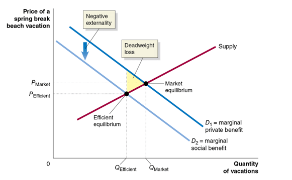
So, in March 2020 there was an externality in consumption from college students taking spring break beach vacations because people in large crowds spread the virus. In other words, the students’ marginal private benefit from being on the beach was greater than the marginal social benefit, taking into account that being on the beach might spread the virus.
The following figure shows the market for spring break beach vacations. The price of a vacation includes transportation costs, renting a hotel room, meals, and any fees to use the beach. Demand curve D1 is the market demand curve and represents the marginal private benefit to students from vacationing on a crowded beach during spring break. But spring breakers don’t bear all the cost of potentially contracting the coronavirus by being on a crowded beach because the cost of their spreading the virus is borne by others. So, there is negative externality from vacationing on the beach equal to the vertical distance between D1, which represents the marginal private benefit, and D2, which represents the marginal social benefit, including the chance of spreading the virus by contracting it on a crowded beach.
Because of the externality, the actual number of people taking spring break beach vacations in March 2020, QMarket, was greater than the efficient number, QEfficient. In Section 5.3 of the Hubbard and O’Brien textbook, we show that when there is an externality in production, a tax equal to the per unit cost of the externality will result in the efficient level of output because the tax causes firms to internalize the externality. In a similar way, a tax on spring break beach vacations equal to the per unit cost of the externality would shift the marginal private benefit curve, D1, down to where it became the same as the marginal social benefit curve, D2. By leading spring breakers to internalize the cost of the externality, the tax would cause the market quantity of beach vacations to decline to the efficient quantity, QEfficient.
In practice, however, imposing a tax on people taking a beach vacation would be difficult for two key reasons: (1) In March 2020, there were many aspects of the coronavirus, including how it spread and its fatality rate, that made calculating the value of the negative externality difficult, and (2) collecting a tax on the many spring breakers crowded on beaches would have been administratively difficult. In the face of these factors, governors and mayors used the command-and-control approach in March of closing beaches, hotels, and restaurants rather than the market-based approach of levying a tax.
Sources: Arian Campo-Flores and Craig Karmin, “The Last Place to be Hit With Coronavirus Worries? Florida Beaches,” Wall Street Journal, March 21, 2020; Aimee Ortiz, “Man Who Said, ‘If I Get Corona, I Get Corona,’ Apologizes,” New York Times, March 24, 2020; and Ryan W. Miller, “’If I Get Corona, I Get Corona’: Coronavirus Pandemic Doesn’t Slow Spring Breakers’ Party,” usatoday.com, March 21, 2020.
Question
According to news reports, some college students on spring break in March 2020 were unaware that partying on the beach put them at risk of contracting the coronavirus. Many also assumed that no one younger than 30 was at risk of becoming seriously ill from the virus, although, in fact, the virus did kill people in their 20s. Suppose that every student on spring break were completely informed about the risks of partying on the beach. Using the figure above, briefly explain how each of the following would have been affected. Draw a graph to illustrate your answer.
a. the demand curve, D1
b. the demand curve, D2
c. QMarket
d. QEfficient
e. PMarket
f. PEfficient
g. Size of the deadweight loss
Instructors can access the answers to these questions by emailing Pearson at christopher.dejohn@pearson.com and stating your name, affiliation, school email address, course number.
Supports: Hubbard/O’Brien, Chapter 24, Money, Banks, and the Federal Reserve System; Macroeconomics Chapter 14; Essentials of Economics Chapter 16.
Apply the Concept: WHAT DO BANK RUNS TELL US ABOUT PANIC TOILET PAPER BUYING DURING THE CORONAVIRUS PANDEMIC?
Here’s the key point: Lack of confidence leads to panic buying, but a return of confidence leads to a return to normal buying.
In Chapter 24, Section 24.4 of the Hubbard and O’Brien Economics 8e text (Chapter 14, Section 14.4 of Macroeconomics 8e) we discuss the problem of bank runs that plagued the U.S. financial system during the years before the Federal Reserve began operations 1914. During the 2020 coronavirus epidemic in the United States consumers bought most of the toilet paper available in supermarkets leaving the shelves bare. Toilet paper runs turn out to be surprisingly similar to bank runs.
First, consider bank runs. The United States, like other countries, has a fractional reserve banking system, which means that banks keep less than 100 percent of their deposits as reserves. During most days, banks will experience roughly the same amount of funds being withdrawn as being deposited. But if, unexpectedly, a large number of depositors simultaneously attempt to withdraw their deposits from a bank, the bank experiences a run that it may not be able to meet with its cash on hand. If large numbers of banks experience runs, the result is a bank panic that can shut down the banking system.
Runs on commercial banks in the United States have effectively ended due to the combination of the Federal Reserve acting as a lender of last resort to banks experiencing runs and the Federal Deposit Insurance Corporation (FDIC) insuring bank deposits (currently up to $250,000 per person, per bank). But consider the situation prior to 1914. As a depositor in a bank during that period, if you had any reason to suspect that your bank was having problems, you had an incentive to be at the front of the line to withdraw your money. Even if you were convinced that your bank was well managed and its loans and investments were sound, if you believed the bank’s other depositors thought the bank had a problem, you still had an incentive to withdraw your money before the other depositors arrived and forced the bank to close. In other words, in the absence of a lender of last resort or deposit insurance, the stability of a bank depends on the confidence of its depositors. In such a situation, if bad news—or even false rumors—shakes that confidence, a bank will experience a run.
Moreover, without a system of government deposit insurance, bad news about one bank can snowball and affect other banks, in a process called contagion. Once one bank has experienced a run, depositors of other banks may become concerned that their banks might also have problems. These depositors have an incentive to withdraw their money from their banks to avoid losing it should their banks be forced to close.
Now think about toilet paper in supermarkets. From long experience, supermarkets, such as Kroger, Walmart, and Giant Eagle, know their usual daily sales and can place orders that will keep their shelves stocked. The same is true of online sites like Amazon. By the same token, manufacturers like Kimberly-Clark and Procter and Gamble, set their production schedules to meet their usual monthly sales. Consumers buy toilet paper as needed, confident that supermarkets will always have some available.
Photo of empty supermarket shelves taken in Boston, MA in March 2020. Credit: Lena Buananno
But then the coronavirus hit and in some states non-essential businesses, colleges, and schools were closed and people were advised to stay home as much as possible. Supermarkets remained open everywhere as did, of course, online sites such as Amazon. But as people began to consider what products they would need if they were to remain at home for several weeks, toilet paper came to mind.
At first only a few people decided to buy several weeks worth of toilet paper at one time, but that was enough to make the shelves holding toilet paper begin to look bare in some supermarkets. As they saw the bare shelves, some people who would otherwise have just bought their usual number of rolls decided that they, too, needed to buy several weeks worth, which made the shelves look even more bare, which inspired more to people to buy several weeks worth, and so on until most supermarkets had sold out of toilet paper, as did Amazon and other online sites.
Before 1914 if you were a bank depositor, you knew that if other depositors were withdrawing their money, you had to withdraw yours before the bank had given out all its cash and closed. In the coronavirus epidemic, you knew that if you failed to rush to the supermarket to buy toilet paper, the supermarket was likely to be sold out when you needed some. Just as banks relied on the confidence of depositors that their money would be available when they wanted to withdraw it, supermarkets rely on the confidence of shoppers that toilet paper and other products will be available to buy when they need them. A loss of that confidence can cause a run on toilet paper just as before 1914 a similar loss of confidence caused runs on banks.
In bank runs, depositors are, in effect, transferring a large part of the country’s inventory of currency out of banks, where it’s usually kept, and into the depositors’ homes. Similarly, during the epidemic, consumers were transferring a large part of the country’s inventory of toilet paper out of supermarkets and into the consumers’ homes. Just as currency is more efficiently stored in banks to be withdrawn only as depositors need it, toilet paper is more efficiently stored in supermarkets (or in Amazon’s warehouses) to be purchased only when consumers need it.
Notice that contagion is even more of a problem in a toilet paper run than in a bank run. People can ordinarily only withdraw funds from banks where they have a deposit, but consumers can buy toilet paper wherever they can find it. And during the epidemic there were news stories of people traveling from store to store—often starting early in the morning—buying up toilet paper.
Finally, should the government’s response to the toilet paper run of 2020 be similar to its response to the bank runs of the 1800s and early 1900s? To end bank runs, Congress established (1) the Fed—to lend banks currency during a run—and (2) the FDIC—to insure deposits, thereby removing a depositor’s fear that the depositor needed to be near the head of the line to withdraw money before the bank’s cash holdings were exhausted.
The situation is different with toilet paper. Supermarkets are eventually able to obtain as much toilet paper as they need from manufacturers. Once production increases enough to restock supermarket shelves, consumers—many of whom already have enough toilet paper to last them several weeks—stop panic buying and ample quantities of toilet paper will be available. Once consumers regain confidence that toilet paper will be available when they need it, they have less incentive to hoard it. Just as a lack of confidence leads to panic buying, a return of confidence leads to a return to normal buying.
Although socialist countries such as Venezuela, Cuba, and North Korea suffer from chronic shortages of many goods, market economies like the United States experience shortages only under unusual circumstances like an epidemic or natural disaster.
Note: For more on bank panics, see Hubbard and O’Brien, Money, Banking, and Financial Markets, 3rd edition, Chapter 12 on which some of this discussion is based.
Sources: Sharon Terlep, “Relax, America: The U.S. Has Plenty of Toilet Paper,” Wall Street Journal, March 16, 2020; Matthew Boyle, “You’ll Get Your Toilet Paper, But Tough Choices Have to Be Made: Grocery CEO,” bloomberg.com, March 18, 2020; and Michael Corkery and Sapna Maheshwari, “Is There Really a Toilet Paper Shortage?” New York Times, March 13, 2020.
Question
Suppose that as a result of their experience during the coronavirus pandemic, the typical household begins to store two weeks worth of toilet paper instead of just a few days worth as they had previously been doing. Will the result be that toilet paper manufacturers permanently increase the quantity of toilet paper that they produce each week?
Instructors can access the answers to these questions by emailing Pearson at christopher.dejohn@pearson.com and stating your name, affiliation, school email address, course number.
Supports: Hubbard/O’Brien, Economics, Chapter 25 – Monetary Policy (Macro Chapter 15 and Essentials Chapter 17), and Chapter 26 – Fiscal Policy (Macro Chapter 16 and Essentials Chapter 18).
The Great Recession of 2007-2009 was the worst economic contraction in the United States since the Great Depression of the 1930s. Accordingly, it brought a vigorous response from federal policymakers. As of late March 2020, it was too soon to tell how severe the economic contraction from the coronavirus pandemic might be. But policymakers had already responded with major initiatives. In the following sections, we compare monetary and fiscal policies employed during the Great Recession and those employed at the beginning of the coronavirus pandemic.
A Brief History of U.S. Recessions
Historically, most recessions in the United States have been caused by one of two often related factors: (1) A financial crisis or (2) Federal Reserve actions taken to reduce the inflation rate. The two main exceptions are the recession of 1973-1975, which was primarily the result of a sharp increase in oil prices, and the recession of 2020, which was the result of the effects of the coronavirus pandemic and of the business closures ordered by state and local governments in an attempt to contain the pandemic.
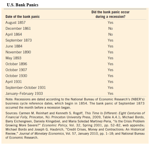
Prior to 1914, the United States lacked both a central bank that could act as a lender of last resort to keep bank runs from escalating into bank panics and a system of deposit insurance. By cutting off many businesses from their main source of credit and cutting off both households and firms from their bank deposits, bank panics resulted in declines in production and employment. The failure of the Federal Reserve to effectively deal with the waves of bank panics from 1930 to 1933 at the beginning of the Great Depression led Congress in 1934 to establish the Federal Deposit Insurance Corporation (FDIC) to insure deposits in commercial banks (currently up to $250,000 per depositor, per bank). The following table shows that prior to World War II (U.S. participation lasted from 1941 to 1945), most recessions were associated with bank panics.
As a result of deposit insurance and more active Federal Reserve discount lending, after World War II problems in the commercial banking system were no longer a major source of instability in the U.S. economy. As the following figure shows, declines in residential construction have preceded every recession in the United States since 1958 (the shaded areas represent periods of recession). Edward Leamer of the University of California, Los Angeles had gone so far as to argue that “housing is the business cycle.” Prior to the housing crash that preceded the Great Recession, the main cause of the declines in residential construction shown in the figure were rising mortgage interest rates, typically due to the Federal Reserve raising its target for the federal funds rate—the interest rate that banks charge each other on overnight loans—in response to increases in the inflation rate.
Monetary Policy during the Great Recession
Both the Great Recession of 2007-2009 and pre-World War II recessions were accompanied by financial panics. Both the Great Recession of 2007-2009 and post-World War II recessions were accompanied by sharp downturns in the housing market.
But the Great Recession differed from earlier recessions two key ways: First, it was caused by problems internal to the housing market rather than the effect on the housing market of contractionary monetary policy; and second, it did not involve commercial banks. Instead, it involved the shadow banking sector of investment banks, money market mutual funds, and insurance companies.
Problems began in the market for mortgage-backed securities—bonds that consisted of mortgages bundled together. The value of the bonds depended on the value of the underlying mortgages. When housing prices began to decline in 2006, borrowers began defaulting on mortgages. Many commercial and investment banks owned these mortgage-backed securities, so the decline in the value of the securities caused these banks to suffer heavy losses. By mid-2007, investors and policymakers became concerned about the decline in the value of mortgage-backed securities and the large losses suffered by commercial and investment banks. Many investors refused to buy mortgage-backed securities, and some investors would buy only bonds issued by the U.S. Treasury.
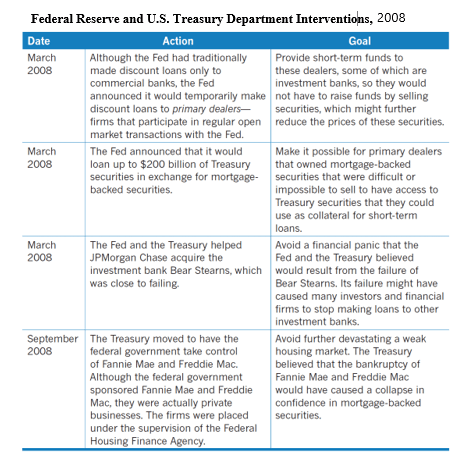
The problems in financial markets resulting from the bursting of the housing bubble were severe, particularly after the failure of the Lehman Brothers investment bank in September 2008. In previous recessions, the focus of the Fed’s expansionary policy had been on cutting its target for the federal funds rate to reduce borrowing costs and spur spending, particularly spending on residential construction. The Fed did rapidly cut its target for the federal funds rate from 5.25 percent in September 2007 to effectively 0 percent in December 2008. But the financial crisis reduced the effect of these rate cuts because the flow of funds through the financial system had largely dried up. As a result, the Fed entered into an unusual partnership with the U.S. Treasury Department and intervened in financial markets in unprecedented ways, which we summarize in the following table. In addition to the actions shown in the table, for the first time since the 1930s, the Fed bought commercial paper—short-term bonds issued by corporations—because many firms found their usual sources of funds were no longer available in the crisis. The Fed’s aim was to restore the flow of funds through the financial system to enable firms to obtain the credit they needed to maintain production and employment.
Fiscal Policy during the Great Recession
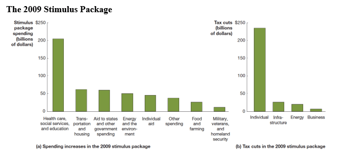
Presidents George W. Bush and Barack Obama both initiated fiscal policy responses to the Great Recession. In 2008, President Bush and Congress enacted a tax cut that took the form of rebates of taxes had already paid. After taking office in January 2009, President Obama and Congress enacted the $840 billion American Recovery and Reinvestment Act (AARA), often called the “stimulus package.” The following figure summarizes the spending and tax cuts in the ARRA.
During the Great Recession, the Fed’s monetary policy moved well beyond its usual focus on targeting the federal funds rate. But fiscal policy was more conventional: Increasing government spending and cutting taxes to increase aggregate demand, real GDP, and employment. The ARRA was notable mainly because of its size.
Monetary Policy in Response to the Coronavirus Epidemic
During 2019, prior to the epidemic beginning to affect the United States, the Fed had twice cut its target for the federal funds rate in response to a slowing rate of economic growth. With the spread of the coronavirus at the start of 2020, the Fed again cut its target twice, returning it effectively to 0 percent in mid-March. With many businesses closed and many consumers largely confined to their homes, the Fed knew that lower borrowing costs would not be the key to maintaining economic activity. Accordingly, the Fed revived some of the lending facilities that it had used during the 2007-2009 financial crisis and set up some new facilities with the goal of maintaining the flow of funds through the financial system and the ability of firms whose revenues had plunged to continue to access credit.
Here is a summary of Fed’s policy actions during March and early April 2020:
Cuts to the Federal Funds Rate The Fed reduced its target for the federal funds rate from a range of 1.75 percent to 1.50 percent to a range of 0 percent to 0.25 percent.
Purchases of Mortgage-Backed Securities To provide funds to the market for mortgage lending, the Fed began purchasing mortgage-backed securities guaranteed by Fannie Mae, Freddie Mac, and Ginnie Mae, which are government-sponsored enterprises (GSEs).
Central Bank Liquidity Swap Lines To meet a surge in demand by foreign businesses and governments for U.S. dollars, the Fed expanded its Central Bank Liquidity Swap Lines, which allow foreign central banks to exchange their currencies for dollars.
Facility for Foreign and International Monetary Authorities To further help foreign central banks meet the demand for U.S. dollars by foreign businesses and governments, the Fed established the Foreign and International Monetary Authorities repurchase agreement facility, which allowed these authorities to “temporarily exchange their U.S. Treasury securities held with the Federal Reserve for U.S. dollars, which can then be made available to institutions in their jurisdictions.” This new facility reduced the need for foreign central banks to sell U.S. Treasury securities to obtain U.S. dollars. Those sales had been contributing to volatility in the market for U.S. Treasury securities.
Primary Dealer Credit Facility To ensure the liquidity of the 24 primary dealers, which are the large financial firms who interact with the Fed in securities markets, the Fed established the Primary Dealer Credit Facility to provide loans to these dealers.
Commercial Paper Funding Facility To ensure that corporations would have access to short-term funds necessary to meet payrolls and pay their suppliers, the Fed established the Commercial Paper Funding Facility to buy commercial paper from corporations.
Primary Market Corporate Credit Facility To ensure that corporations have access to longer-term funds, the Fed established the Primary Market Corporate Credit Facility to make loans to corporations whose bonds are rated investment grade by Moody’s, S&P, and Fitch, the private bond rating agencies.
Secondary Market Corporate Credit Facility To ensure the smooth functioning of the corporate bond market, the Fed established the Secondary Market Corporate Credit Facility to buy in the secondary market investment grade bonds issued by corporations and to buy shares in exchange-traded funds that are primarily invested in such bonds. First established in March, the facility was expanded in April to allow for the purchase of some non-investment grade corporate bonds and the purchase of shares in exchange-traded funds that are invested in such bonds.
Term Asset-Backed Securities Loan Facility (TALF) To support the flow of credit to consumers and businesses, the Fed began buying asset-backed securities (ABS) backed by student loans, auto loans, credit card loans, loans guaranteed by the Small Business Administration (SBA).
Municipal Liquidity Facility To support the ability of state, county, and city governments to borrow, the Fed began buying short-term state and local bonds.
Main Street New Loan Facility (MSNLF) and Main Street Expanded Loan Facility (MSELF) To ensure that small and medium size businesses had the financial resources to survive the crisis, the Fed offered 4-year loans to companies employing up to 10,000 workers or with revenues of less than $2.5 billion. Principal and interest payments were deferred for one year. The facility was intended to augment the Paycheck Protection Programs, which was part of the CARES act and involves loans administered through the federal government’s Small Business Administration to firms with 500 or fewer employees.
In taking these actions, the Fed relied on its authority under Section 13(3) of the Federal Reserve Act, which authorizes the Fed under “unusual and exigent circumstances” to lend broadly. Following the 2007-2009 financial crisis, Congress amended the Federal Reserve Act to require that the Fed receive the prior approval for such actions from the Secretary of the Treasury. After consultation with Fed Chair Jerome Powell, Treasury Secretary Steven Munchin provided the required approval. As in the 2007-2009 financial crisis, the Fed was again conducting monetary policy in collaboration with the U.S. Treasury, rather than operating independently, as it had prior to 2007.
It remains to be seen whether these extraordinary actions will be sufficient to keep funds flowing through the financial system and to provide sufficient credit to allow businesses whose revenues had plunged to remain solvent.
Fiscal Policy in Response to the Coronavirus Epidemic
During the week of March 15, 2020, more than 3 million workers applied for federal unemployment benefits—five times more than had ever previously applied during a single week. Congress and President Donald Trump responded to the crisis by passing three aid packages by the end of March 2020, with the likelihood that further aid packages would be passed during the following weeks.
Unlike with fiscal policy actions during previous recessions, including the ARRA passed during the Great Recession, the main goal of these aid packages was not to directly stimulate aggregate demand by increasing government spending and cutting taxes. With many businesses closed and people in some states being asked to “shelter in place” or stay home except for essential trips such as buying groceries, a stimulus package of the conventional type was unlikely to be effective. Congress and the president instead focused on (1) helping businesses to remain open after many had experienced enormous declines in revenue and (2) providing households with sufficient funds to pay their rent or mortgage, buy groceries, and cover other essential spending.
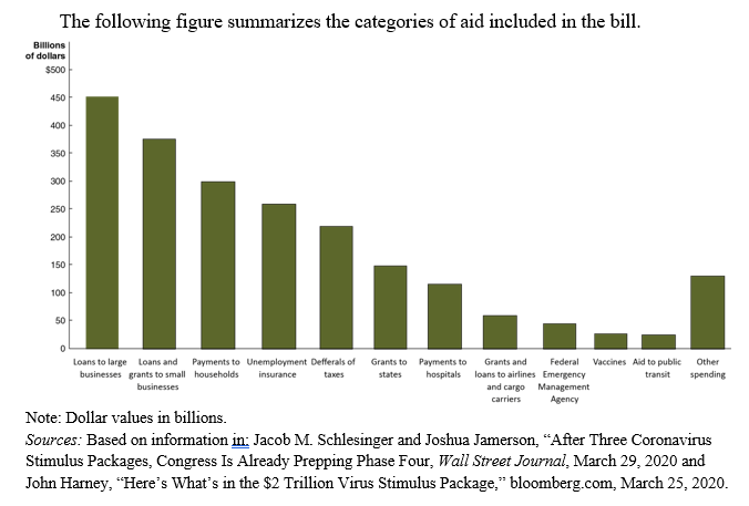
Here is a summary of Congress and the president’s first three fiscal policy actions:
Research Funding and Aid to State and Local Governments In early March, Congress and the president passed an $8.3 billion bill to provide funds for research into a vaccine for the coronavirus and for state and local governments to help cover some of their costs in fighting the virus.
Increases in Benefits and Tax Credits In mid-March, Congress and the president passed a $100 billion bill aimed at increasing unemployment benefits, increasing benefits under the Supplemental Nutrition Assistance Program ( also called food stamps), and providing tax credits to firms offering paid sick leave to employees.
Coronavirus Aid, Relief and Economic Security (CARES) Act On March 27, Congress and the president passed the Coronavirus Aid, Relief and Economic Security (CARES) Act, a more than $2 trillion aid package—by far the largest fiscal policy action in U.S. history—to provide:
Direct payments to households
Supplemental unemployment insurance payments
Funds to state governments to offset some of their costs in fighting in the epidemic
Loans and grants to businesses
The macroeconomic policy actions undertaken by the Fed, Congress, and the president in the spring of 2020 were unprecedented in size and scope. Whether they would be effective in keeping the coronavirus epidemic from causing a major recession in the United States remains to be seen.
Note: Some of the figures and tables reproduced here were first published in Hubbard and O’Brien, Economics, 6th and 8th editions or Hubbard and O’Brien, Money, Banking, and Financial Markets, 3rd edition.
Sources: Federal Reserve Bank of New York, “New York Fed Actions Related to COVID-19,” newyorkfed.org; Board of Governors of the Federal Reserve System, “Text of the Federal Reserve Act: Section 13. Powers of Federal Reserve Banks,” federalreserve.gov, February 13, 2017; Nick Timiraos, “Fed Cuts Rates to Near Zero and Will Relaunch Bond-Buying Program,” Wall Street Journal, March 26, 2020; Eric Morath, Jon Hilsenrath and Sarah Chaney, “Record Rise in Unemployment Claims Halts Historic Run of Job Growth,” Wall Street Journal, March 18, 2020; Emily Cochrane, “House Passes $8.3 Billion Emergency Coronavirus Response Bill,” New York Times, March 9, 2020; and John Harney, “Here’s What’s in the $2 Trillion Virus Stimulus Package,” bloomberg.com, March 25, 2020.
Questions
1. There are both similarities and differences between monetary policies employed during the Great Recession of 2007-2009 and those employed at the beginning of the coronavirus pandemic in 2020.
(a) How has the Fed attempted to stimulate the economy during a typical recession?
(b) Briefly discuss ways in which the Fed’s approach during the Great Recession and during the coronavirus pandemic was similar.
(c) Briefly discuss ways in which the Fed’s approach during the Great Recession and during the coronavirus pandemic differed.
2. There are both similarities and differences between fiscal policies employed during the Great Recession of 2007 – 2009 and those employed at the beginning of the coronavirus pandemic of 2020.
(a) How have Congress and the president attempted to stimulate the economy during a typical recession?
(b) Briefly discuss ways in which Congress and the president’s approach during the Great Recession and during the coronavirus pandemic was similar to traditional expansionary policy.
(c) Briefly discuss how Congress and the president’s approach during the Great Recession and during the coronavirus pandemic differed from traditional expansionary policy.
Instructors can access the answers to these questions by emailing Pearson at christopher.dejohn@pearson.com and stating your name, affiliation, school email address, course number.
Supports: Hubbard/O’Brien, Chapter 23, Aggregate Demand and Aggregate Supply Analysis; Macroeconomics Chapter 13; Essentials of Economics Chapter 15.
Apply the Concept: Using the Aggregate Demand and Aggregate Supply Model to Analyze the Coronavirus Pandemic
Here’s the key point: The coronavirus caused large shifts in short-run aggregate supply and in aggregate demand, so this virus caused by far the largest decline in real GDP and largest increase in unemployment over such a brief period in U.S. history.
In early 2020, the United States experienced an epidemic from a novel coronavirus that causes the disease Covid-19. We can use the aggregate demand and aggregate supply model to analyze some of the key macroeconomic effects on the U.S. economy from this epidemic. As we’ve seen, economists distinguish between recessions caused by an aggregate supply shock, such as an unexpected increase in oil prices, or an aggregate demand shock, such as a decline in spending on new houses. The effects of the coronavirus combined both an aggregate supply shock and an aggregate demand shock.
To this point, we have discussed negative aggregate supply shocks that shift only the short-run aggregate supply curve to the left, leaving the aggregate demand curve unaffected. It’s usually reasonable to assume that the aggregate demand curve doesn’t shift when analyzing the effects of the two main types of supply shocks: (1) a supply shock caused by an increase in the cost of producing goods and services; or (2) a supply shock that reduces the capacity of firms to produce goods and services.
An example of the first type of supply shock is an increase in oil prices. Higher oil prices increase the cost of producing many goods and services, shifting the short-run aggregate supply curve to the left. (See panel (a) of Figure 23.7 in the Hubbard and O’Brien 8th edition text). Total spending in the economy declines, which we show as a movement along the aggregate demand curve (not as a shift in the aggregate demand curve). That movement is the result of the higher price level reducing the spending of households and firms on consumption, investment, and net exports.
The second type of supply shock reduces the capacity of firms and is typically the result of a natural disaster such as the Tohoku earthquake that Japan experienced in 2011. The earthquake triggered a tsunami that disabled the nuclear power plant in the city of Fukushima. The disruption in the power supply to several cities, including Tokyo took months to resolve. During this period, the ability of many Japanese firms to produce goods and services was reduced, causing the short-run aggregate supply curve to shift to the left. Notice that a natural disaster will also have some effect on aggregate demand if there are deaths (about 16,000 people in Japan died as a result of the Tohoku earthquake and tsunami) or if some firms are physically destroyed, making their workers unemployed, thereby reducing the workers’ incomes and their consumption spending. But because the resulting shift of the aggregate demand curve is likely to be small relative to the shift in the short-run aggregate supply curve, it makes sense to concentrate on the effects of the shift in short-run aggregate supply.
The coronavirus pandemic was an unprecedented supply shock to the U.S. economy. The virus originated in the city of Wuhan in China. A number of U.S. firms rely on Chinese suppliers in the Wuhan area. In January 2020, as the government of China closed factories in that area to control the spread of the virus, some U.S. firms, including Apple and Nike, announced that they would be unable to meet their production goals because some of their suppliers had shut down. By March, as the virus began to become widespread in the United States, governors in a number of states ordered all non-essential firms to close.
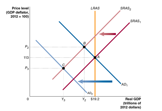
The following figure illustrates the effects of the virus on U.S. real GDP and the price level. In the figure, at the beginning of 2020, the economy was in long-run macroeconomic equilibrium, with the short-run aggregate supply curve, SRAS1, intersecting the aggregate demand curve, AD1, at point A on the long-run aggregate supply curve, LRAS. Equilibrium occurred at real GDP of $19.2 trillion and a price level of 113. By disrupting the global supply chains of U.S. firms and by leading governments to order the closure of many businesses, the virus caused the short-run aggregate supply curve to shift to the left from SRAS1 to SRAS2. (Note that in the following discussion, we are using the basic aggregate demand and aggregate supply model. In this model, there is no economic growth, so the long-run aggregate supply curve (LRAS) doesn’t shift.)
If the virus had caused a supply shock of the first type that we described earlier—affecting the economy in a way similar to a large increase in oil prices—the new short-run equilibrium would have occurred at point B. Real GDP would have declined from $19.2 trillion to Y2 and the price level would have risen from 113 to P2. (We prepared this content and graph in early April, so we don’t yet know the full effects of the virus on the economy. We therefore don’t attempt to put actual values on the new short-run equilibrium real GDP and price level.)
But point B was not the new short-run equilibrium for several reasons:
Reduced consumption spending The government closed many businesses, directly reducing output resulting in millions of workers losing their jobs. As workers experienced falling incomes, they reduced their consumption spending.
Reduced investmentspending Many residential and business construction projects had to be suspended, reducing investment spending.
Reduced exports U.S. exports declined because the pandemic also led to closures of businesses in Europe, Canada, Japan, and other U.S. trading partners.
As a result of these factors, the United States experienced a sharp decline in total spending in the economy, shifting the aggregate demand curve to the left from AD1 to AD2. In analyzing the supply shock resulting from the coronavirus, we have to include the effect on aggregate demand, which we ignore when considering supply shocks caused by higher oil prices or by a natural disaster, such as an earthquake.
Because the coronavirus pandemic caused both the SRAS and the AD curves to shift to the left, the new short-run equilibrium occurred at point C, with real GDP having fallen to Y3 and the price level having declined to P3. Note that if the shift of the SRAS curve had been larger than the shift of the AD curve, real GDP would have fallen further and the price level would have risen, rather than fallen.
The coronavirus pandemic resulted in very large shifts in short-run aggregate supply and in aggregate demand, so this virus caused by far the largest decline in real GDP and largest increase in unemployment over such a brief period in the history of the United States. The U.S. economy also suffered a large decline in real GDP and a substantial increase in unemployment during the Great Depression of the 1930s. But the decline in the U.S. economy during that economic contraction had been stretched out over the period from August 1929 to March 1933, rather than happening suddenly as was true with the contraction caused by the coronavirus.
Sources: Ruth Simon and Austen Hufford, “Not Just Nike and Apple: Small U.S. Firms Disrupted by Coronavirus,” Wall Street Journal, February 21, 2020; Eric Morath, Jon Hilsenrath, and Sarah Chaney, “Record 3.28 Million File for U.S. Jobless Benefits,” Wall Street Journal, March 26, 2020; and “158 Million Americans Told to Stay Home, but Trump Pledges to Keep It Short,” New York Times, March 26, 2020.
Question
During the spring of 2020, many state and local governments ordered most non-essential businesses to close. Suppose that, as a result, the short-run aggregate supply curve, SRAS, shifted to the left by more than did the aggregate demand curve, AD. On the graph shown here, draw in a new SRAS given this assumption. Label this curve SRAS3. Label the new equilibrium level of real GDP Y4 and the new equilibrium price level P4. Briefly explain the relationship between Y3 and Y4 and between P3 and P4, as shown in your graph.
Instructors can access the answers to these questions by emailing Pearson at christopher.dejohn@pearson.com and stating your name, affiliation, school email address, course number.
Supports: Hubbard/O’Brien, Chapter 4, Economic Efficiency, Government Price Setting, and Taxes
Apply the Concept: Should the Government Limit Price Gouging in an Emergency?
Here’s the key point: In the long run, the market will respond to an increase in demand by increasing supply without an increase in price, but in the short run consumers as a group lose from a sharp increase in price.
In early 2020, the coronavirus epidemic spread through many countries, including the United States. The Centers for Disease Control encouraged people to thoroughly wash their hands and disinfect surfaces to help slow the spread of the virus. People flooded supermarkets and pharmacies to buy hand sanitizer, disinfectant wipes, and toilet paper. By March, these products had largely disappeared from store shelves. People who hoped to buy them on Amazon or eBay found that sellers were charging prices far above normal.
For instance, sellers on Amazon were charging $99.95 for large bottles of hand sanitizer that normally sell for $9.95. One seller was even charging $459 for a two-ounce bottle! Such large increases in the prices of essential goods, particularly during an emergency, is called price gouging and is against the law in 34 states. Many people consider price gouging immoral because it makes it difficult for people to afford essential goods during an emergency. During the coronavirus epidemic, using hand sanitizer was an important safety measure when people lacked easy access to soap and water. (Note: A list of state price gouging laws as of March 25, 2020 can be found here: https://consumer.findlaw.com/consumer-transactions/price-gouging-laws-by-state.html)
Laws against price gouging are essentially price ceilings set at the price of a good before the emergency began. Recall that a price ceiling is a legally determined maximum price that sellers may charge. What economic effect do price gouging laws have? It’s useful to distinguish the very short run, during which it isn’t possible to produce more of the good, and the medium run when additional production is possible.
The effect of price gouging laws in the very short run
The following graph shows the market for hand sanitizer in the very short run of a few weeks. Assume that the price of an 8-ounce bottle of hand sanitizer prior to the arrival of the coronavirus epidemic in the United States was $3.99. The normal level of demand is shown as demand curve, D1. In the very short run, the supply of hand sanitizer is fixed at the quantity, Q1, currently available at retail stores and on online sites such as Amazon. We show this fixed quantity as the vertical supply curve, S.
The increased demand for hand sanitizer resulting from the epidemic shifts the demand curve to the right from D1 to D2. In the absence of price gouging laws, the price will rise from $3.99 to a higher price, which we’ll assume is $9.99. Laws against price gouging (assuming they are enforced) will impose a price ceiling at $3.99. The result of the price ceiling is a shortage equal to the difference between the new quantity demanded, Q2, and the fixed supply Q1. The price ceiling results in consumers receiving consumer surplus equal to the area below demand curve D2 and above the price of $3.99, shown in the figure as the sum of A and B. If there is no price ceiling and the equilibrium price rises to $9.99, area B will become part of producer surplus, reducing consumer surplus to just area A. Sellers have gained from the higher price at the expense of buyers.
Remember, though, that in a market system prices play an important role in directing resources to their most valuable use. If the equilibrium price rises to $9.99, at point A on D2, the marginal benefit from the last bottle of sanitizer sold is equal to its price, which is the economically efficient outcome. With the imposition of a price ceiling, some buyers whose marginal benefits are represented by the values along D2 between point A and point B may buy bottles of sanitizer while some buyers with a higher marginal benefit may be unable to. Consider a bus driver or police officer who does not have easy access to soap and water. These people would have been willing to pay $9.99 for sanitizer but may be unable to find any because of the shortage resulting from the price ceiling. Now consider someone who spends most of his or her time at home or who already has a supply of hand sanitizer and would be unwilling to buy a bottle at a price of $9.99 decides to do so at a price of $3.99.
Someone with a low income may have greater difficulty paying $9.99 than would someone with a high income and so, holding everything else constant, we might expect that without a price ceiling more high-income people will be able to buy sanitizer than will low-income people. This consideration leads many people to support laws against price gouging even if they know that the laws reduce economic efficiency.
The effect of price gouging laws in the medium run
The following figure shows the more familiar situation when the time period is long enough for firms to increase production of hand sanitizer. (Note that this figure is similar to Figure 4.9 in the Hubbard and O’Brien textbook.) In this case, as demand shifts to the right from D1 to D2 because of the epidemic, in the absence of a price ceiling, the price will increase from $3.99 per bottle to $5.99 per bottle and the equilibrium quantity of bottles will increase from Q1 to Q3.
The supply curve, S, is upward sloping because we would expect that firms’ marginal cost of producing sanitizer will increase as they expand output. For example, in March 2020, an article in the Wall Street Journal described how EO Products, located in San Rafael, California, quadrupled its output of hand sanitizer by “running extra shifts, speeding up lines, hiring temporary workers and converting factory lines designed for other products to make hand sanitizer instead.” These actions made it possible for EO to increase the quantity of sanitizer it supplied, but meant that its marginal cost of production was increasing.
A price gouging law that kept the price of hand sanitizer fixed at $3.99 per bottle would result in the quantity of sanitizer supplied remaining at Q1, causing a shortage equal to the difference between Q2 and Q1. Note that the price ceiling eliminates the incentive for firms to increase production of sanitizer. Because marginal cost is increasing, firms will ordinarily need to receive a higher price in order to increase production. In fact, though, that EO Products President Tom Feegel decided not to raise his price despite the firm’s higher cost: “Raising prices at this time would not be in alignment with our core values.”
The price ceiling causes consumer surplus to increase by the area of rectangle A and fall by the area of rectangle B. Rectangle A would have been part of producer surplus in the absence of the price ceiling. In that sense, the price ceiling benefits buyers at the expense of sellers. Compared with the situation in which the price is allowed to rise to $5.99, producer surplus declines by the area of A plus the area of C. The areas of triangles B and C represent deadweight loss or the reduction in economic surplus resulting from the imposition of the price ceiling resulting from the price gouging law.
We can summarize the effects of the price gouging law shown in the figure:
Consumers who are able to buy the sanitizer at the ceiling price of $3.99 gain.
Consumers who would be able to buy the sanitizer at the equilibrium price $5.99 but are unable to find any at the ceiling price of $3.99 lose.
Sellers experience a loss of producer surplus.
Economy efficiency is reduced by an amount equal to the deadweight loss.
What happens in the market for hand sanitizer in the long run?
Suppose that the demand for hand sanitizer permanently increases as a result of the coronavirus epidemic because many people decide that it is now worthwhile to routinely sanitize their hands. In that case, we would expect to see an increase quantity of bottles of hand sanitizer sold with price ending up back at the original price of $3.99. Why wouldn’t the price need to be permanently higher? Remember that we expect the marginal cost of producing a good to increase as a firm produces more of a good during a given period of time.
For instance, if EO products has to pay workers a higher hourly wage to work more than 8 hours per day or hires new workers who initially aren’t as skilled at producing sanitizer, the company’s marginal cost will increase. But over time EO’s new workers will become more familiar with their jobs and the company will be able to hire enough workers so that none will have to work more than 8 hours per day. We would expect that EO’s marginal cost of producing sanitizer will eventually fall back to $3.99 per bottle and that the same will be true for other firms in the industry. As a result, the price declines back to $3.99.
In addition, the price increase to $5.99 may give other firms an incentive to begin producing hand sanitizer. If more firms enter the industry, in the long run, the supply curve for hand sanitizer will shift to the right, which will contribute to bringing the price back down to $3.99. In general, in the long run the market will respond to an increase in demand by increasing supply without an increase in price.
Sources: Sharon Terlep, “One Company’s Hands-On Effort to Ramp Up Sanitizer Production,” Wall Street Journal, March 16, 2020; Sharon Terlep, “Amazon Dogged by Price Gouging as Coronavirus Fears Grow,” Wall Street Journal, March 5, 2020; and Jack Nicas, “The Man With 17,700 Bottles of Hand Sanitizer Just Donated Them,” New York Times, March 15, 2020.
Questions
Many state laws against price gouging apply only during emergencies.
Why might state governments decide that the laws should apply during emergencies rather than at all times?
What protects consumers from price gouging during times that aren’t emergencies?
Instructors can access the answers to these questions by emailing Pearson at christopher.dejohn@pearson.com and stating your name, affiliation, school email address, course number.
On March 19th Glenn Hubbard sat down with the editorial team at Pearson to talk through some of the high-level economic issues involved in the coronavirus pandemic.
In this 10 minute podcast Glenn discusses the nature of the economic shock and what we should expect, based on historical shocks. We explore every day topics students are wondering about like what will the job market look like to the policy ideas of what could help stabilize the US economy.
Give your students the link and ask them any of the following discussion questions to get them thinking about the pandemic in an economic context:
1. Is this kind of economic supply shock a new concept or something that the U.S. has experienced before? Is there any precedent for whether this should be a short or drawn out recession? What factors will contribute to the length of the recession?
2. What economic policies would you prescribe for dealing with this crisis and why? Which policy would be the most beneficial for families given the current state of the economy? Which policies would be the most beneficial for businesses and long-term economic growth?
3. What current mandates as a result of the pandemic could translate into longer-term modifications to how we learn and work? Discuss the possible structural changes to the economy.
4. What are the trade-offs involved in controlling the pandemic? Assuming there will be a significant impact on the economy, what macroeconomic policies would you implement to soften the shock to allow people to more easily follow the guidelines to reduce the pandemic without suffering severe economic consequences? Will your policies help restart the economy once the pandemic has passed?
Instructors can access the answers to these questions by emailing Pearson at Christopher.dejohn@pearson.com and stating your name, affiliation, school email address, course number.