COVID-19 Update: Monetary and Fiscal Policy Responses: The Great Recession vs. the Coronavirus Pandemic

Supports:  Hubbard/O’Brien, Economics, Chapter 25 – Monetary Policy (Macro Chapter 15 and Essentials Chapter 17), and Chapter 26 – Fiscal Policy (Macro Chapter 16 and Essentials Chapter 18).

The Great Recession of 2007-2009 was the worst economic contraction in the United States since the Great Depression of the 1930s.  Accordingly, it brought a vigorous response from federal policymakers.  As of late March 2020, it was too soon to tell how severe the economic contraction from the coronavirus pandemic might be.  But policymakers had already responded with major initiatives.  In the following sections, we compare monetary and fiscal policies employed during the Great Recession and those employed at the beginning of the coronavirus pandemic.

A Brief History of U.S. Recessions

             Historically, most recessions in the United States have been caused by one of two often related factors: (1) A financial crisis or (2) Federal Reserve actions taken to reduce the inflation rate.  The two main exceptions are the recession of 1973-1975, which was primarily the result of a sharp increase in oil prices, and the recession of 2020, which was the result of the effects of the coronavirus pandemic and of the business closures ordered by state and local governments in an attempt to contain the pandemic.

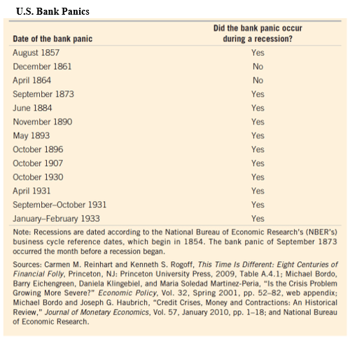
            Prior to 1914, the United States lacked both a central bank that could act as a lender of last resort to keep bank runs from escalating into bank panics and a system of deposit insurance.  By cutting off many businesses from their main source of credit and cutting off both households and firms from their bank deposits, bank panics resulted in declines in production and employment. The failure of the Federal Reserve to effectively deal with the waves of bank panics from 1930 to 1933 at the beginning of the Great Depression led Congress in 1934 to establish the Federal Deposit Insurance Corporation (FDIC) to insure deposits in commercial banks (currently up to $250,000 per depositor, per bank). The following table shows that prior to World War II (U.S. participation lasted from 1941 to 1945), most recessions were associated with bank panics.

 As a result of deposit insurance and more active Federal Reserve discount lending, after World War II problems in the commercial banking system were no longer a major source of instability in the U.S. economy.  As the following figure shows, declines in residential construction have preceded every recession in the United States since 1958 (the shaded areas represent periods of recession). Edward Leamer of the University of California, Los Angeles had gone so far as to argue that “housing is the business cycle.” Prior to the housing crash that preceded the Great Recession, the main cause of the declines in residential construction shown in the figure were rising mortgage interest rates, typically due to the Federal Reserve raising its target for the federal funds rate—the interest rate that banks charge each other on overnight loans—in response to increases in the inflation rate.


Monetary Policy during the Great Recession

Both the Great Recession of 2007-2009 and pre-World War II recessions were accompanied by financial panics.  Both the Great Recession of 2007-2009 and post-World War II recessions were accompanied by sharp downturns in the housing market.

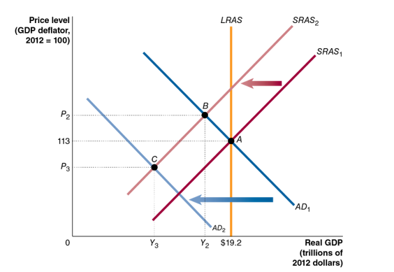
But the Great Recession differed from earlier recessions two key ways:  First, it was caused by problems internal to the housing market rather than the effect on the housing market of contractionary monetary policy; and second, it did not involve commercial banks.  Instead, it involved the shadow banking sector of investment banks, money market mutual funds, and insurance companies. 

            Problems began in the market for mortgage-backed securities—bonds that consisted of mortgages bundled together. The value of the bonds depended on the value of the underlying mortgages. When housing prices began to decline in 2006, borrowers began defaulting on mortgages.  Many commercial and investment banks owned these mortgage-backed securities, so the decline in the value of the securities caused these banks to suffer heavy losses. By mid-2007, investors and policymakers became concerned about the decline in the value of mortgage-backed securities and the large losses suffered by commercial and investment banks. Many investors refused to buy mortgage-backed securities, and some investors would buy only bonds issued by the U.S. Treasury.

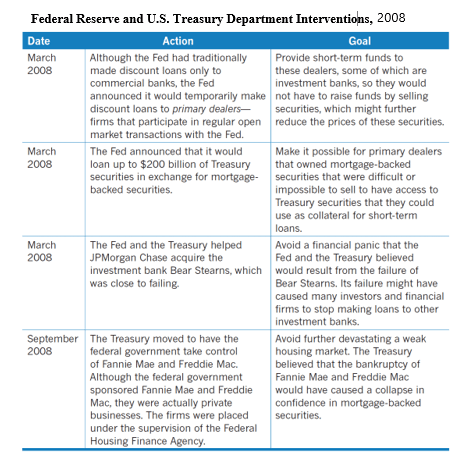
            The problems in financial markets resulting from the bursting of the housing bubble were severe, particularly after the failure of the Lehman Brothers investment bank in September 2008.  In previous recessions, the focus of the Fed’s expansionary policy had been on cutting its target for the federal funds rate to reduce borrowing costs and spur spending, particularly spending on residential construction.  The Fed did rapidly cut its target for the federal funds rate from 5.25 percent in September 2007 to effectively 0 percent in December 2008. But the financial crisis reduced the effect of these rate cuts because the flow of funds through the financial system had largely dried up.  As a result, the Fed entered into an unusual partnership with the U.S. Treasury Department and intervened in financial markets in unprecedented ways, which we summarize in the following table. In addition to the actions shown in the table, for the first time since the 1930s, the Fed bought commercial paper—short-term bonds issued by corporations—because many firms found their usual sources of funds were no longer available in the crisis. The Fed’s aim was to restore the flow of funds through the financial system to enable firms to obtain the credit they needed to maintain production and employment.


Fiscal Policy during the Great Recession

Presidents George W. Bush and Barack Obama both initiated fiscal policy responses to the Great Recession. In 2008, President Bush and Congress enacted a tax cut that took the form of rebates of taxes had already paid. After taking office in January 2009, President Obama and Congress enacted the $840 billion American Recovery and Reinvestment Act (AARA), often called the “stimulus package.”  The following figure summarizes the spending and tax cuts in the ARRA.

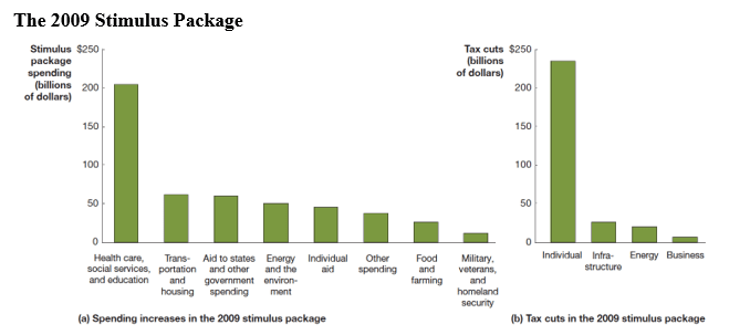
During the Great Recession, the Fed’s monetary policy moved well beyond its usual focus on targeting the federal funds rate. But fiscal policy was more conventional: Increasing government spending and cutting taxes to increase aggregate demand, real GDP, and employment. The ARRA was notable mainly because of its size.

Monetary Policy in Response to the Coronavirus Epidemic

            During 2019, prior to the epidemic beginning to affect the United States, the Fed had twice cut its target for the federal funds rate in response to a slowing rate of economic growth.  With the spread of the coronavirus at the start of 2020, the Fed again cut its target twice, returning it effectively to 0 percent in mid-March.  With many businesses closed and many consumers largely confined to their homes, the Fed knew that lower borrowing costs would not be the key to maintaining economic activity.  Accordingly, the Fed revived some of the lending facilities that it had used during the 2007-2009 financial crisis and set up some new facilities with the goal of maintaining the flow of funds through the financial system and the ability of firms whose revenues had plunged to continue to access credit.

            Here is a summary of Fed’s policy actions during March and early April 2020:

  • Cuts to the Federal Funds Rate  The Fed reduced its target for the federal funds rate from a range of 1.75 percent to 1.50 percent to a range of 0 percent to 0.25 percent.
  • Purchases of Mortgage-Backed Securities  To provide funds to the market for mortgage lending, the Fed began purchasing mortgage-backed securities guaranteed by Fannie Mae, Freddie Mac, and Ginnie Mae, which are government-sponsored enterprises (GSEs).
  • Central Bank Liquidity Swap Lines  To meet a surge in demand by foreign businesses and governments for U.S. dollars, the Fed expanded its Central Bank Liquidity Swap Lines, which allow foreign central banks to exchange their currencies for dollars.
  • Facility for Foreign and International Monetary Authorities  To further help foreign central banks meet the demand for U.S. dollars by foreign businesses and governments, the Fed established the Foreign and International Monetary Authorities repurchase agreement facility, which allowed these authorities to “temporarily exchange their U.S. Treasury securities held with the Federal Reserve for U.S. dollars, which can then be made available to institutions in their jurisdictions.” This new facility reduced the need for foreign central banks to sell U.S. Treasury securities to obtain U.S. dollars. Those sales had been contributing to volatility in the market for U.S. Treasury securities.
  • Primary Dealer Credit Facility  To ensure the liquidity of the 24 primary dealers, which are the large financial firms who interact with the Fed in securities markets, the Fed established the Primary Dealer Credit Facility to provide loans to these dealers.
  • Commercial Paper Funding Facility  To ensure that corporations would have access to short-term funds necessary to meet payrolls and pay their suppliers, the Fed established the Commercial Paper Funding Facility to buy commercial paper from corporations.
  • Primary Market Corporate Credit Facility  To ensure that corporations have access to longer-term funds, the Fed established the Primary Market Corporate Credit Facility to make loans to corporations whose bonds are rated investment grade by Moody’s, S&P, and Fitch, the private bond rating agencies.
  • Secondary Market Corporate Credit Facility  To ensure the smooth functioning of the corporate bond market, the Fed established the Secondary Market Corporate Credit Facility to buy in the secondary market investment grade bonds issued by corporations and to buy shares in exchange-traded funds that are primarily invested in such bonds. First established in March, the facility was expanded in April to allow for the purchase of some non-investment grade corporate bonds and the purchase of shares in exchange-traded funds that are invested in such bonds.
  • Term Asset-Backed Securities Loan Facility (TALF) To support the flow of credit to consumers and businesses, the Fed began buying asset-backed securities (ABS) backed by student loans, auto loans, credit card loans, loans guaranteed by the Small Business Administration (SBA).
  • Municipal Liquidity Facility To support the ability of state, county, and city governments to borrow, the Fed began buying short-term state and local bonds.
  • Main Street New Loan Facility (MSNLF) and Main Street Expanded Loan Facility (MSELF) To ensure that small and medium size businesses had the financial resources to survive the crisis, the Fed offered 4-year loans to companies employing up to 10,000 workers or with revenues of less than $2.5 billion. Principal and interest payments were deferred for one year. The facility was intended to augment the Paycheck Protection Programs, which was part of the CARES act and involves loans administered through the federal government’s Small Business Administration to firms with 500 or fewer employees.

In taking these actions, the Fed relied on its authority under Section 13(3) of the Federal Reserve Act, which authorizes the Fed under “unusual and exigent circumstances” to lend broadly.  Following the 2007-2009 financial crisis, Congress amended the Federal Reserve Act to require that the Fed receive the prior approval for such actions from the Secretary of the Treasury. After consultation with Fed Chair Jerome Powell, Treasury Secretary Steven Munchin provided the required approval.  As in the 2007-2009 financial crisis, the Fed was again conducting monetary policy in collaboration with the U.S. Treasury, rather than operating independently, as it had prior to 2007.

It remains to be seen whether these extraordinary actions will be sufficient to keep funds flowing through the financial system and to provide sufficient credit to allow businesses whose revenues had plunged to remain solvent. 

Fiscal Policy in Response to the Coronavirus Epidemic

            During the week of March 15, 2020, more than 3 million workers applied for federal unemployment benefits—five times more than had ever previously applied during a single week.  Congress and President Donald Trump responded to the crisis by passing three aid packages by the end of March 2020, with the likelihood that further aid packages would be passed during the following weeks.

            Unlike with fiscal policy actions during previous recessions, including the ARRA passed during the Great Recession, the main goal of these aid packages was not to directly stimulate aggregate demand by increasing government spending and cutting taxes. With many businesses closed and people in some states being asked to “shelter in place” or stay home except for essential trips such as buying groceries, a stimulus package of the conventional type was unlikely to be effective. Congress and the president instead focused on (1) helping businesses to remain open after many had experienced enormous declines in revenue and (2) providing households with sufficient funds to pay their rent or mortgage, buy groceries, and cover other essential spending.

Here is a summary of Congress and the president’s first three fiscal policy actions:

  • Research Funding and Aid to State and Local Governments In early March, Congress and the president passed an $8.3 billion bill to provide funds for research into a vaccine for the coronavirus and for state and local governments to help cover some of their costs in fighting the virus.
  • Increases in Benefits and Tax Credits  In mid-March, Congress and the president passed a $100 billion bill aimed at increasing unemployment benefits, increasing benefits under the Supplemental Nutrition Assistance Program ( also called food stamps), and providing tax credits to firms offering paid sick leave to employees.
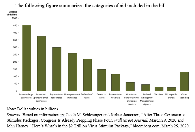
  • Coronavirus Aid, Relief and Economic Security (CARES) Act  On March 27, Congress and the president passed the Coronavirus Aid, Relief and Economic Security (CARES) Act, a more than $2 trillion aid package—by far the largest fiscal policy action in U.S. history—to provide:
    • Direct payments to households
    • Supplemental unemployment insurance payments
    • Funds to state governments to offset some of their costs in fighting in the epidemic
    • Loans and grants to businesses

The macroeconomic policy actions undertaken by the Fed, Congress, and the president in the spring of 2020 were unprecedented in size and scope. Whether they would be effective in keeping the coronavirus epidemic from causing a major recession in the United States remains to be seen.

Note: Some of the figures and tables reproduced here were first published in Hubbard and O’Brien, Economics, 6th and 8th editions or Hubbard and O’Brien, Money, Banking, and Financial Markets, 3rd edition.

Sources: Federal Reserve Bank of New York, “New York Fed Actions Related to COVID-19,” newyorkfed.org; Board of Governors of the Federal Reserve System, “Text of the Federal Reserve Act: Section 13. Powers of Federal Reserve Banks,” federalreserve.gov, February 13, 2017; Nick Timiraos, “Fed Cuts Rates to Near Zero and Will Relaunch Bond-Buying Program,” Wall Street Journal, March 26, 2020; Eric Morath, Jon Hilsenrath and Sarah Chaney, “Record Rise in Unemployment Claims Halts Historic Run of Job Growth,” Wall Street Journal, March 18, 2020; Emily Cochrane, “House Passes $8.3 Billion Emergency Coronavirus Response Bill,” New York Times, March 9, 2020; and John Harney, “Here’s What’s in the $2 Trillion Virus Stimulus Package,” bloomberg.com, March 25, 2020.

Questions 

1. There are both similarities and differences between monetary policies employed during the Great Recession of 2007-2009 and those employed at the beginning of the coronavirus pandemic in 2020.

(a) How has the Fed attempted to stimulate the economy during a typical recession? 

(b) Briefly discuss ways in which the Fed’s approach during the Great Recession and during the coronavirus pandemic was similar.

(c) Briefly discuss ways in which the Fed’s approach during the Great Recession and during the coronavirus pandemic differed.

2.  There are both similarities and differences between fiscal policies employed during the Great Recession of 2007 – 2009 and those employed at the beginning of the coronavirus pandemic of 2020.

(a) How have Congress and the president attempted to stimulate the economy during a typical recession?

(b) Briefly discuss ways in which Congress and the president’s approach during the Great Recession and during the coronavirus pandemic was similar to traditional expansionary policy.

(c) Briefly discuss how Congress and the president’s approach during the Great Recession and during the coronavirus pandemic differed from traditional expansionary policy.

Instructors can access the answers to these questions by emailing Pearson at christopher.dejohn@pearson.com and stating your name, affiliation, school email address, course number.

COVID-19 Update: Applying the AD and AS Analysis

Supports:  Hubbard/O’Brien, Chapter 23, Aggregate Demand and Aggregate Supply Analysis; Macroeconomics Chapter 13; Essentials of Economics Chapter 15.

Apply the Concept: Using the Aggregate Demand and Aggregate Supply Model to Analyze the Coronavirus Pandemic

Here’s the key point:   The coronavirus caused large shifts in short-run aggregate supply and in aggregate demand, so this virus caused by far the largest decline in real GDP and largest increase in unemployment over such a brief period in U.S. history.

In early 2020, the United States experienced an epidemic from a novel coronavirus that causes the disease Covid-19. We can use the aggregate demand and aggregate supply model to analyze some of the key macroeconomic effects on the U.S. economy from this epidemic. As we’ve seen, economists distinguish between recessions caused by an aggregate supply shock, such as an unexpected increase in oil prices, or an aggregate demand shock, such as a decline in spending on new houses.  The effects of the coronavirus combined both an aggregate supply shock and an aggregate demand shock.

 To this point, we have discussed negative aggregate supply shocks that shift only the short-run aggregate supply curve to the left, leaving the aggregate demand curve unaffected. It’s usually reasonable to assume that the aggregate demand curve doesn’t shift when analyzing the effects of the two main types of supply shocks: (1) a supply shock caused by an increase in the cost of producing goods and services; or (2) a supply shock that reduces the capacity of firms to produce goods and services.

            An example of the first type of supply shock is an increase in oil prices. Higher oil prices increase the cost of producing many goods and services, shifting the short-run aggregate supply curve to the left. (See panel (a) of Figure 23.7 in the Hubbard and O’Brien 8th edition text). Total spending in the economy declines, which we show as a movement along the aggregate demand curve (not as a shift in the aggregate demand curve).  That movement is the result of the higher price level reducing the spending of households and firms on consumption, investment, and net exports.

The second type of supply shock reduces the capacity of firms and is typically the result of a natural disaster such as the Tohoku earthquake that Japan experienced in 2011. The earthquake triggered a tsunami that disabled the nuclear power plant in the city of Fukushima. The disruption in the power supply to several cities, including Tokyo took months to resolve. During this period, the ability of many Japanese firms to produce goods and services was reduced, causing the short-run aggregate supply curve to shift to the left. Notice that a natural disaster will also have some effect on aggregate demand if there are deaths (about 16,000 people in Japan died as a result of the Tohoku earthquake and tsunami) or if some firms are physically destroyed, making their workers unemployed, thereby reducing the workers’ incomes and their consumption spending.  But because the resulting shift of the aggregate demand curve is likely to be small relative to the shift in the short-run aggregate supply curve, it makes sense to concentrate on the effects of the shift in short-run aggregate supply.

The coronavirus pandemic was an unprecedented supply shock to the U.S. economy. The virus originated in the city of Wuhan in China. A number of U.S. firms rely on Chinese suppliers in the Wuhan area.  In January 2020, as the government of China closed factories in that area to control the spread of the virus, some U.S. firms, including Apple and Nike, announced that they would be unable to meet their production goals because some of their suppliers had shut down. By March, as the virus began to become widespread in the United States, governors in a number of states ordered all non-essential firms to close. 

The following figure illustrates the effects of the virus on U.S. real GDP and the price level. In the figure, at the beginning of 2020, the economy was in long-run macroeconomic equilibrium, with the short-run aggregate supply curve, SRAS1, intersecting the aggregate demand curve, AD1, at point A on the long-run aggregate supply curve, LRAS. Equilibrium occurred at real GDP of $19.2 trillion and a price level of 113. By disrupting the global supply chains of U.S. firms and by leading governments to order the closure of many businesses, the virus caused the short-run aggregate supply curve to shift to the left from SRAS1 to SRAS2. (Note that in the following discussion, we are using the basic aggregate demand and aggregate supply model. In this model, there is no economic growth, so the long-run aggregate supply curve (LRAS) doesn’t shift.)

If the virus had caused a supply shock of the first type that we described earlier—affecting the economy in a way similar to a large increase in oil prices—the new short-run equilibrium would have occurred at point B.  Real GDP would have declined from $19.2 trillion to Y2 and the price level would have risen from 113 to P2. (We prepared this content and graph in early April, so we don’t yet know the full effects of the virus on the economy.  We therefore don’t attempt to put actual values on the new short-run equilibrium real GDP and price level.)

            But point B was not the new short-run equilibrium for several reasons: 

  1. Reduced consumption spending  The government closed many businesses, directly reducing output resulting in millions of workers losing their jobs. As workers experienced falling incomes, they reduced their consumption spending.
  2. Reduced investment spending  Many residential and business construction projects had to be suspended, reducing investment spending.
  3. Reduced exports  U.S. exports declined because the pandemic also led to closures of businesses in Europe, Canada, Japan, and other U.S. trading partners.

As a result of these factors, the United States experienced a sharp decline in total spending in the economy, shifting the aggregate demand curve to the left from AD1 to AD2. In analyzing the supply shock resulting from the coronavirus, we have to include the effect on aggregate demand, which we ignore when considering supply shocks caused by higher oil prices or by a natural disaster, such as an earthquake.

            Because the coronavirus pandemic caused both the SRAS and the AD curves to shift to the left, the new short-run equilibrium occurred at point C, with real GDP having fallen to Y3 and the price level having declined to P3. Note that if the shift of the SRAS curve had been larger than the shift of the AD curve, real GDP would have fallen further and the price level would have risen, rather than fallen.

            The coronavirus pandemic resulted in very large shifts in short-run aggregate supply and in aggregate demand, so this virus caused by far the largest decline in real GDP and largest increase in unemployment over such a brief period in the history of the United States.   The U.S. economy also suffered a large decline in real GDP and a substantial increase in unemployment during the Great Depression of the 1930s. But the decline in the U.S. economy during that economic contraction had been stretched out over the period from August 1929 to March 1933, rather than happening suddenly as was true with the contraction caused by the coronavirus.

Sources: Ruth Simon and Austen Hufford, “Not Just Nike and Apple: Small U.S. Firms Disrupted by Coronavirus,” Wall Street Journal, February 21, 2020; Eric Morath, Jon Hilsenrath, and Sarah Chaney, “Record 3.28 Million File for U.S. Jobless Benefits,” Wall Street Journal, March 26, 2020; and “158 Million Americans Told to Stay Home, but Trump Pledges to Keep It Short,” New York Times, March 26, 2020.


Question 

During the spring of 2020, many state and local governments ordered most non-essential businesses to close. Suppose that, as a result, the short-run aggregate supply curve, SRAS, shifted to the left by more than did the aggregate demand curve, AD. On the graph shown here, draw in a new SRAS given this assumption. Label this curve SRAS3. Label the new equilibrium level of real GDP Y4 and the new equilibrium price level P4. Briefly explain the relationship between Y3 and Y4 and between P3 and P4, as shown in your graph. 

Instructors can access the answers to these questions by emailing Pearson at christopher.dejohn@pearson.com and stating your name, affiliation, school email address, course number.

Freakonomics Podcast: Is $2 Trillion the Right Medicine for a Sick Economy?

Hear Glenn Hubbard with Stephen Dubner on a recent Freakonomics Podcast. Glenn and other economists discuss the fiscal response to the COVID-19 economic crisis. https://freakonomics.com/podcast/covid-19-cares-act/

SMALL BUSINESS ALONE NEEDS $1 TRILLION NOW

From Bloomberg Opinion – coauthored by Michael Strain & Glenn Hubbard – from March 20th, 2020

https://www.bloomberg.com/opinion/articles/2020-03-20/small-business-needs-1-trillion-now-for-coronavirus-relief?srnd=opinion

SMALL BUSINESS ALONE NEEDS $1 TRILLION NOW- from Bloomberg Opinion – coauthored by Michael Strain & Glenn Hubbard. The GOP stimulus plan has good ideas for covering service-industry payrolls amid the coronavirus shutdown, but doesn’t set aside enough to pay for it.

A BUSINESS FISCAL RESPONSE TO THE COVID-19 RECESSION

From the American Enterprise Institute – March 20th, 2020

https://www.aei.org/wp-content/uploads/2020/03/hubbard-strain.pdf

A business fiscal response to the COVID-19 Recession – from the American Enterprise Institute – co-authored by R. Glenn Hubbard & Michael R. Strain, Director of Economic Policy Studies at AEI.

COVID-19 Update: Should the Government Limit Price Gouging in an Emergency?

Supports:  Hubbard/O’Brien, Chapter 4, Economic Efficiency, Government Price Setting, and Taxes

Apply the Concept: Should the Government Limit Price Gouging in an Emergency?

Here’s the key point:   In the long run, the market will respond to an increase in demand by increasing supply without an increase in price, but in the short run consumers as a group lose from a sharp increase in price.

In early 2020, the coronavirus epidemic spread through many countries, including the United States.   The Centers for Disease Control encouraged people to thoroughly wash their hands and disinfect surfaces to help slow the spread of the virus.   People flooded supermarkets and pharmacies to buy hand sanitizer, disinfectant wipes, and toilet paper.  By March, these products had largely disappeared from store shelves.  People who hoped to buy them on Amazon or eBay found that sellers were charging prices far above normal.

 For instance, sellers on Amazon were charging $99.95 for large bottles of hand sanitizer that normally sell for $9.95. One seller was even charging $459 for a two-ounce bottle!  Such large increases in the prices of essential goods, particularly during an emergency, is called price gouging and is against the law in 34 states. Many people consider price gouging immoral because it makes it difficult for people to afford essential goods during an emergency.  During the coronavirus epidemic, using hand sanitizer was an important safety measure when people lacked easy access to soap and water.  (Note: A list of state price gouging laws as of March 25, 2020 can be found here: https://consumer.findlaw.com/consumer-transactions/price-gouging-laws-by-state.html)

            Laws against price gouging are essentially price ceilings set at the price of a good before the emergency began. Recall that a price ceiling is a legally determined maximum price that sellers may charge.  What economic effect do price gouging laws have?  It’s useful to distinguish the very short run, during which it isn’t possible to produce more of the good, and the medium run when additional production is possible.

The effect of price gouging laws in the very short run

The following graph shows the market for hand sanitizer in the very short run of a few weeks.  Assume that the price of an 8-ounce bottle of hand sanitizer prior to the arrival of the coronavirus epidemic in the United States was $3.99.  The normal level of demand is shown as demand curve, D1. In the very short run, the supply of hand sanitizer is fixed at the quantity, Q1, currently available at retail stores and on online sites such as Amazon. We show this fixed quantity as the vertical supply curve, S.

The increased demand for hand sanitizer resulting from the epidemic shifts the demand curve to the right from D1 to D2. In the absence of price gouging laws, the price will rise from $3.99 to a higher price, which we’ll assume is $9.99.  Laws against price gouging (assuming they are enforced) will impose a price ceiling at $3.99.  The result of the price ceiling is a shortage equal to the difference between the new quantity demanded, Q2, and the fixed supply Q1.  The price ceiling results in consumers receiving consumer surplus equal to the area below demand curve D2 and above the price of $3.99, shown in the figure as the sum of A and B. If there is no price ceiling and the equilibrium price rises to $9.99, area B will become part of producer surplus, reducing consumer surplus to just area A.  Sellers have gained from the higher price at the expense of buyers.

Remember, though, that in a market system prices play an important role in directing resources to their most valuable use.  If the equilibrium price rises to $9.99, at point A on D2, the marginal benefit from the last bottle of sanitizer sold is equal to its price, which is the economically efficient outcome.  With the imposition of a price ceiling, some buyers whose marginal benefits are represented by the values along D2 between point A and point B may buy bottles of sanitizer while some buyers with a higher marginal benefit may be unable to.  Consider a bus driver or police officer who does not have easy access to soap and water.  These people would have been willing to pay $9.99 for sanitizer but may be unable to find any because of the shortage resulting from the price ceiling. Now consider someone who spends most of his or her time at home or who already has a supply of hand sanitizer and would be unwilling to buy a bottle at a price of $9.99 decides to do so at a price of $3.99.

Someone with a low income may have greater difficulty paying $9.99 than would someone with a high income and so, holding everything else constant, we might expect that without a price ceiling more high-income people will be able to buy sanitizer than will low-income people. This consideration leads many people to support laws against price gouging even if they know that the laws reduce economic efficiency.

The effect of price gouging laws in the medium run

            The following figure shows the more familiar situation when the time period is long enough for firms to increase production of hand sanitizer.  (Note that this figure is similar to Figure 4.9 in the Hubbard and O’Brien textbook.) In this case, as demand shifts to the right from D1 to D2 because of the epidemic, in the absence of a price ceiling, the price will increase from $3.99 per bottle to $5.99 per bottle and the equilibrium quantity of bottles will increase from Q1 to Q3.  

The supply curve, S, is upward sloping because we would expect that firms’ marginal cost of producing sanitizer will increase as they expand output. For example, in March 2020, an article in the Wall Street Journal described how EO Products, located in San Rafael, California, quadrupled its output of hand sanitizer by “running extra shifts, speeding up lines, hiring temporary workers and converting factory lines designed for other products to make hand sanitizer instead.” These actions made it possible for EO to increase the quantity of sanitizer it supplied, but meant that its marginal cost of production was increasing.

            A price gouging law that kept the price of hand sanitizer fixed at $3.99 per bottle would result in the quantity of sanitizer supplied remaining at Q1, causing a shortage equal to the difference between Q2 and Q1.  Note that the price ceiling eliminates the incentive for firms to increase production of sanitizer. Because marginal cost is increasing, firms will ordinarily need to receive a higher price in order to increase production. In fact, though, that EO Products President Tom Feegel decided not to raise his price despite the firm’s higher cost: “Raising prices at this time would not be in alignment with our core values.”

The price ceiling causes consumer surplus to increase by the area of rectangle A and fall by the area of rectangle B. Rectangle A would have been part of producer surplus in the absence of the price ceiling. In that sense, the price ceiling benefits buyers at the expense of sellers. Compared with the situation in which the price is allowed to rise to $5.99, producer surplus declines by the area of A plus the area of C. The areas of triangles B and C represent deadweight loss or the reduction in economic surplus resulting from the imposition of the price ceiling resulting from the price gouging law.

We can summarize the effects of the price gouging law shown in the figure:

  1. Consumers who are able to buy the sanitizer at the ceiling price of $3.99 gain.
  2. Consumers who would be able to buy the sanitizer at the equilibrium price $5.99 but are unable to find any at the ceiling price of $3.99 lose.
  3. Sellers experience a loss of producer surplus.
  4. Economy efficiency is reduced by an amount equal to the deadweight loss.

What happens in the market for hand sanitizer in the long run?

            Suppose that the demand for hand sanitizer permanently increases as a result of the coronavirus epidemic because many people decide that it is now worthwhile to routinely sanitize their hands.  In that case, we would expect to see an increase quantity of bottles of hand sanitizer sold with price ending up back at the original price of $3.99. Why wouldn’t the price need to be permanently higher? Remember that we expect the marginal cost of producing a good to increase as a firm produces more of a good during a given period of time.

For instance, if EO products has to pay workers a higher hourly wage to work more than 8 hours per day or hires new workers who initially aren’t as skilled at producing sanitizer, the company’s marginal cost will increase. But over time EO’s new workers will become more familiar with their jobs and the company will be able to hire enough workers so that none will have to work more than 8 hours per day. We would expect that EO’s marginal cost of producing sanitizer will eventually fall back to $3.99 per bottle and that the same will be true for other firms in the industry. As a result, the price declines back to $3.99.

In addition, the price increase to $5.99 may give other firms an incentive to begin producing hand sanitizer. If more firms enter the industry, in the long run, the supply curve for hand sanitizer will shift to the right, which will contribute to bringing the price back down to $3.99.  In general, in the long run the market will respond to an increase in demand by increasing supply without an increase in price.

Sources: Sharon Terlep, “One Company’s Hands-On Effort to Ramp Up Sanitizer Production,” Wall Street Journal, March 16, 2020; Sharon Terlep, “Amazon Dogged by Price Gouging as Coronavirus Fears Grow,” Wall Street Journal, March 5, 2020; and Jack Nicas, “The Man With 17,700 Bottles of Hand Sanitizer Just Donated Them,” New York Times, March 15, 2020.

Questions

Many state laws against price gouging apply only during emergencies.

  1. Why might state governments decide that the laws should apply during emergencies rather than at all times?
  2. What protects consumers from price gouging during times that aren’t emergencies?

Instructors can access the answers to these questions by emailing Pearson at christopher.dejohn@pearson.com and stating your name, affiliation, school email address, course number.

Coronavirus Pandemic & the Economy: An Overview

On March 19th Glenn Hubbard sat down with the editorial team at Pearson to talk through some of the high-level economic issues involved in the coronavirus pandemic.

In this 10 minute podcast Glenn discusses the nature of the economic shock and what we should expect, based on historical shocks. We explore every day topics students are wondering about like what will the job market look like to the policy ideas of what could help stabilize the US economy.

Give your students the link and ask them any of the following discussion questions to get them thinking about the pandemic in an economic context:

1. Is this kind of economic supply shock a new concept or something that the U.S. has experienced before? Is there any precedent for whether this should be a short or drawn out recession? What factors will contribute to the length of the recession?

2. What economic policies would you prescribe for dealing with this crisis and why? Which policy would be the most beneficial for families given the current state of the economy? Which policies would be the most beneficial for businesses and long-term economic growth?

3. What current mandates as a result of the pandemic could translate into longer-term modifications to how we learn and work? Discuss the possible structural changes to the economy.

4. What are the trade-offs involved in controlling the pandemic? Assuming there will be a significant impact on the economy, what macroeconomic policies would you implement to soften the shock to allow people to more easily follow the guidelines to reduce the pandemic without suffering severe economic consequences? Will your policies help restart the economy once the pandemic has passed?

Instructors can access the answers to these questions by emailing Pearson at Christopher.dejohn@pearson.com and stating your name, affiliation, school email address, course number.

Here for You

Professors’ and students’ lives have been turned upside down as a result of what’s going on with the Coronavirus pandemic. Courses which have traditionally been taught in the classroom with maybe some online components are now completely virtual. We empathize with professors who are being thrown into an online environment without much help.

That’s why now was the right time to start this blog and create a series of podcasts. What is written/recorded here isn’t perfect and hasn’t been put through the rounds of review our textbook goes through. But this is timely. And it is an effort to help bring the current situation in the world into your classroom in a way that you can easily share with students and incorporate in your coursework in an online environment.

We hope these posts and podcasts do the job to help in this unprecedented time. And we want to hear from you if there’s more we can be doing, or if there’s something specific you’d like us to cover. Please reach out at our contact page!