Supports: Macroeconomics, Chapter 9,Economics, Chapter 19, and Essentials of Economics, Chapter 13.
Image generated by GTP-4o.
In its “Employment Situation” report for July 2024, the Bureau of Labor Statistics (BLS) stated that according to the household survey the total number of people employed, the total number of people unemployed, and the unemployment rate all increased. Would we expect this result to always hold? That is, in a month in which both the total number of people employed and the total number of people unemployed increased will the unemployment rate always increase? Briefly explain.
Solving the Problem Step 1: Review the chapter material. This problem is about calculating the unemployment rate, so you may want to review Chapter 9, Section 9.1, “Measuring the Unemployment Rate, the Labor Force Participation Rate, and the Employment-Population Ratio.”
Step 2: Answer the question by explaining whether we can be certain what happens to the unemployment rate in a month in which both the total number of people employed and the total number of people unemployed increased. The unemployment rate is equal to the number of people unemployed divided by the number of people in the labor force (multiplied by 100). The labor force equals the sum of the number of people employed and the number of people unemployed.
Suppose, for example, that the unemployment rate in the previous month was 4 percent. If both the number of people employed and the number of people unemployed increase, the unemployment rate will increase if the increase in the number of people unemployed as a percentage of the increase in the labor force is greater than 4 percent. The unemployment rate will decrease if the increase in the number of people unemployed as a percentage of the increase in the labor force is less than 4 percent.
Consider a simple numerical example. Suppose that in the previous month there were 96 people employed and 4 people unemployed. In that case, the unemployment rate will be (4/(96 + 4)) x 100 = 4.0%.
Suppose that during the month the number of people employed increases by 30 and the number of people unemployed increases by 1. In that case, there are now 126 people employed and 5 people unemployed. The unemployment rate will have fallen from 4.0% to (5/(126 + 5)) x 100 = 3.8%.
Now suppose that the number of people employed increased by 30 and the number of people unemployed increases by 3. The unemployment will have risen from 4.0% to (7/(126 + 7)) x 100 = 5.3%.
We can conclude that what happened in July 2024 need not always happen. If both the total number of people employed and the total number of people unemployed increased during a given month, we can’t be sure whether the unemployment rate has increased or decreased.
Earlier this week, as we discussed in this blog post, the Federal Reserve’s policy-making Federal Open Market Committee (FOMC) voted to leave its target for the federal funds rate unchanged. In his press conference following the meeting, Fed Chair Jerome Powell stated that: “Overall, a broad set of indicators suggests that conditions in the labor market have returned to about where they stood on the eve of the pandemic—strong but not overheated.”
This morning (August 2), the Bureau of Labor Statistics (BLS) released its “Employment Situation” report (often referred to as the “jobs report”) for July, which indicates that the labor market may be weaker than Powell and the other members of the FOMC believed it to be when they decided to leave their target for the federal funds rate unchanged.
The jobs report has two estimates of the change in employment during the month: one estimate from the establishment survey, often referred to as the payroll survey, and one from the household survey. As we discuss in Macroeconomics, Chapter 9, Section 9.1 (Economics, Chapter 19, Section 19.1), many economists and policymakers at the Federal Reserve believe that employment data from the establishment survey provides a more accurate indicator of the state of the labor market than do either the employment data or the unemployment data from the household survey. (The groups included in the employment estimates from the two surveys are somewhat different, as we discuss in this post.)
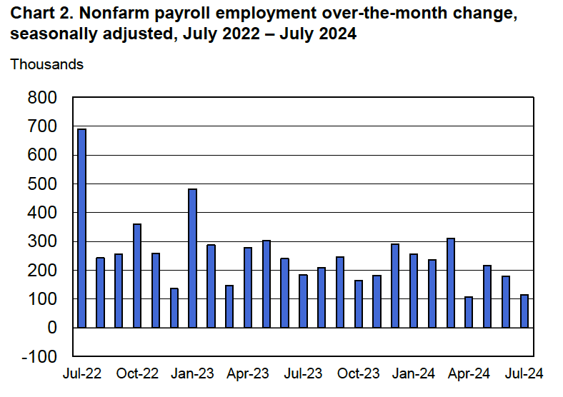
According to the establishment survey, there was a net increase of 114,000 jobs during July. This increase was below the increase of 175,000 to 185,000 that economists had forecast in surveys by the Wall Street Journal and bloomberg.com. The following figure, taken from the BLS report, shows the monthly net changes in employment for each month during the past two years.
The previously reported increases in employment for April and May were revised downward by 29,000 jobs. (The BLS notes that: “Monthly revisions result from additional reports received from businesses and government agencies since the last published estimates and from the recalculation of seasonal factors.”) As we’ve discussed in previous posts (most recently here), downward revisions to the payroll employment estimates are particularly likely at the beginning of a recession, although this month’s adjustments were relatively small.
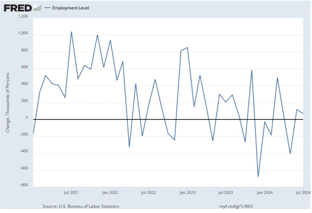
As the following figure shows, the net change in jobs from the household survey moves much more erratically than does the net change in jobs in the establishment survey. The net change in jobs as measured by the household survey declined from 116,000 in June to 67,000 in June. So, in this case the direction of change in the two surveys was the same—a decline in the increase in the number of jobs.
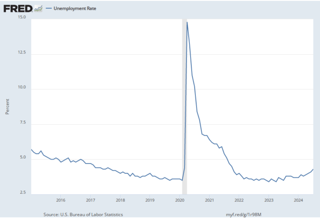
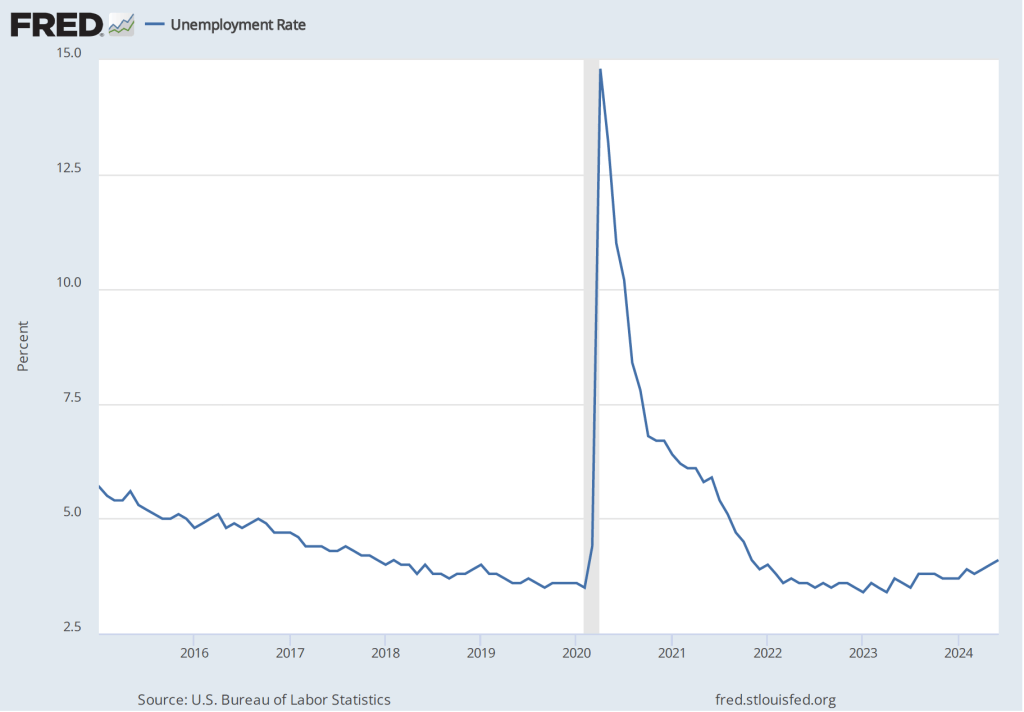
As the following figure shows, the unemployment rate, which is also reported in the household survey, increased from 4.1 percent to 4.3 percent—the highest unemployment rate since October 2021. Although still low by historical standards, July was the fifth consecutive month in which the unemployment rate increased. It is also higher than the unemployment rate just before the pandemic. The unemployment rate was below 4 percent most months from mid-2018 to early 2020.
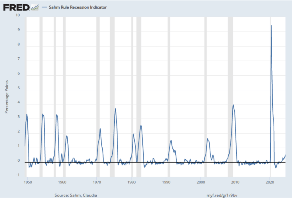
Some economists and policymakers have been following the Sahm rule, named after Claudia Sahm Chief Economist for New Century Advisors and a former Fed economist. The Sahm rule, as stated on the site of the Federal Reserve Bank of St. Louis is: “Sahm Recession Indicator signals the start of a recession when the three-month moving average of the national unemployment rate (U3 [measure]) rises by 0.50 percentage points or more relative to the minimum of the three-month averages from the previous 12 months.” The following figure shows the values of this indicator dating back to March 1949.
So, according to this indicator, the U.S. economy is now at the start of a recession. Does that mean that a recession has actually started? Not necessarily. As Sahm stated in an interview this morning, her indicator is a historical relationship that may not always hold, particularly given how signficantly the labor market has been affected during the last four years by the pandemic.
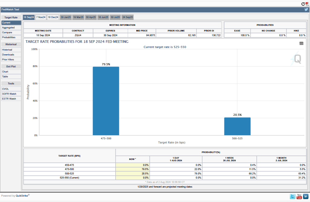
As we noted in a post earlier this week, investors who buy and sell federal funds futures contracts assigned a probability of 11 percent that the FOMC would cut its target for the federal funds rate by 0.50 percentage point at its next meeting. (Investors in this market assigned a probability of 89 percent that the FOMC would cut its target by o.25 percentage point.) Today, investors dramatically increased the probability to 79.5 percent of a 0.50 cut in the federal funds rate target, as shown in this figure from the CME site.
Investors on the stock market appear to believe that the probability of a recession beginning before the end of the year has increased, as indicated by sharp declines today in the stock market indexes.
The next scheduled FOMC meeting isn’t until September 17-18. The FOMC is free to meet in between scheduled meetings but doing so might be interpreted as meanng that economy is in crisis, which is a message the committee is unlikely to want to send. It would likely take additional unfavorable reports on macro data for the FOMC not to wait until September to take action on cutting its target for the federal funds rate.
Image of “Federal Reserve Chair Jerome Powell speaking at a podium” generated by GTP-4o.
At the conclusion of its July 30-31 meeting, the Federal Reserve’s policy-making Federal Open Market Committee (FOMC) voted unamiously to leave its target range for the federal funds rate unchanged at 5.25 percent to 5.5 percent. (The statement the FOMC issued following the meeting can be found here.)
In the statement Fed Chair Jerome Powell read at the beginning of his press conference after the meeting, Powell appeared to be repeating a position he has stated in speeches and interviews during the past month:
“We have stated that we do not expect it will be appropriate to reduce the target range for the federal funds rate until we have gained greater confidence that inflation is moving sustainably toward 2 percent. The second-quarter’s inflation readings have added to our confidence, and more good data would further strengthen that confidence. We will continue to make our decisions meeting by meeting.”
But in answering questions from reporters, he made it clear that—as many economists and Wall Street investors had already concluded—the FOMC was likely to reduce its target for the federal funds rate at its next meeting on September 17-18. Powell noted that recent data were consistent with the inflation rate continuing to decline toward the Fed’s 2 percent annual target. Powell summarized the consensus from the discussion among committee members as being that “the time was approaching for cutting rates.”
Futures markets allow investors to buy and sell futures contracts on commodities–such as wheat and oil–and on financial assets. Investors can use futures contracts both to hedge against risk—such as a sudden increase in oil prices or in interest rates—and to speculate by, in effect, betting on whether the price of a commodity or financial asset is likely to rise or fall. (We discuss the mechanics of futures markets in Chapter 7, Section 7.3 of Money, Banking, and the Financial System.) The CME Group was formed from several futures markets, including the Chicago Mercantile Exchange, and allows investors to trade federal funds futures contracts. The data that result from trading on the CME indicate what investors in financial markets expect future values of the federal funds rate to be. The following chart from the CME’s FedWatch Tool shows the current values resulting from trading of federal funds futures.
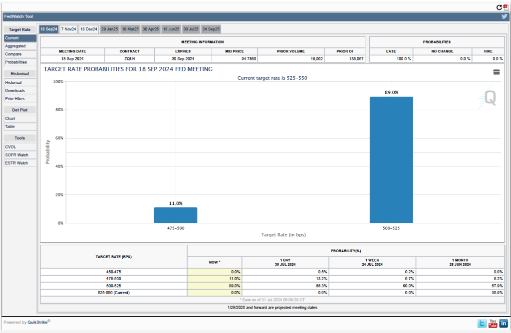
The probabilities in the chart reflect investors’ predictions of what the FOMC’s target for the federal funds rate will be after the committee’s September meeting. The chart indicates that investors assign a probability of 100 percent to the FOMC cutting its federal funds rate target at this meeting. Investors assign a probability of 89.0 percent that the committee will cut its target by 0.25 percentage point and a probability of 11.0 percent that the commitee will cut its target by 0.50 percentage point. When asked at his press conference whether the committee had given any consideration to making a 0.50 percentage point cut in its target, Powell said that it hadn’t.
Powell stated that the latest data on wage increases had led the committee to conclude that the labor market was no longer a source of inflationary pressure. The morning of the press conference, the Bureau of Labor Statistics (BLS) released its latest report on the Employment Cost Index (ECI). As we’ve noted in earlier posts, as a measure of the rate of increase in labor costs, the FOMC prefers the ECI to average hourly earnings (AHE).
As a measure of how wages are increasing or decreasing during a particular period, AHE can suffer from composition effects because AHE data aren’t adjusted for changes in the mix of occupations workers are employed in. In contrast, the ECI holds the mix of occupations constant. The ECI does have the drawback that it is only available quarterly whereas the AHE is available monthly.
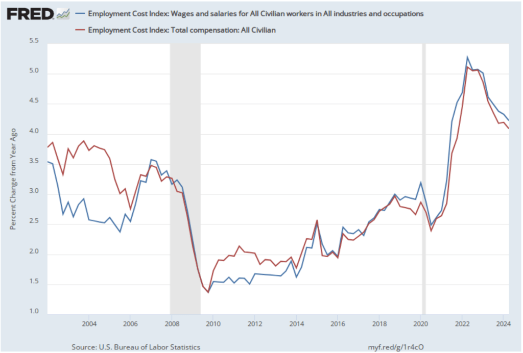
The following figure shows the percentage change in the ECI for all civilian workers from the same quarter in the previous year. The blue line looks only at wages and salaries, while the red line is for total compensation, including non-wage benefits like employer contributions to health insurance. The rate of increase in the wage and salary measure decreased slightly from 4.3 percent in the first quarter of 2024 to 4.2 percent in the second quarter of 2024. The rate of increase in compensation also declined slightly from 4.2 percent to 4.1 percent. As the figure shows, both measures continued their declines from the peak of wage inflation during the second quarter of 2022. In his press conference, Powell said that the this latest ECI report was a little better than the committee had expected.
Finally, Powell noted that the committee saw no indication that the U.S. economy was heading for a recession. He observed that: “The labor market has come into better balance and the unemployment rate remains low.” In addition, he said that output continued to grow steadily. In particular, he pointed to growth in real final sales to private domestic purchasers. This macro variable equals the sum of personal consumption expenditures and gross private fixed investment. By excluding exports, government purchases, and changes in inventories, final sales to private domestic purchasers removes the more volatile components of gross domestic product and provides a better measure of the underlying trend in the growth of output.
As the following figure shows, this measure of output has grown at an annual rate of more than 2.5 percent in each of the last three quarters. Output expanding at that rate is indicative of an economy that is neither overheating nor heading toward a recession.
At this point, unless macro data releases are unexpectedly strong or weak during the next six weeks, it seems nearly certain that at its September meeting the FOMC will reduce its target range for the federal funds rate by 0.25 percentage point.
Federal Reserve Chair Jerome Powell at a press conference following a meeting of the Federal Open Market Committee (Photo from federal reserve.gov)
Inflation in 2024 is a tale of two quarters. During the first quarter of 2024, inflation ran higher than expected considering the falling inflation rates at the end of 2023. As a result, although at the beginning of the year many economists and Wall Street analysts had expected the Federal Reserve’s policy-making Federal Open Market Committee (FOMC) would cut its target for the federal funds rate at least once in the first half of 2024, the FOMC left its target unchanged.
On July 26, the Bureau of Economic Analysis (BEA) released its “Personal Income and Outlays” report for June. The report includes monthly data on the personal consumption expenditures (PCE) price index. The Fed relies on annual changes in the PCE price index to evaluate whether it’s meeting its 2 percent annual inflation target. The report confirmed that PCE inflation slowed in the second quarter, bringing it closer to the Fed’s 2 percent target.
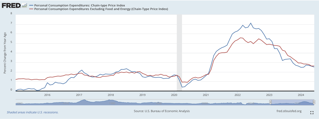
The following figure shows PCE inflation (blue line) and core PCE inflation (red line)—which excludes energy and food prices—for the period since January 2015 with inflation measured as the percentage change in the PCE from the same month in the previous year. Measured this way, in June PCE inflation (the blue line) was 2.5 percent, down slightly from PCE inflation of 2.6 percent in May. Core PCE inflation (the red line) in June was also 2.5 percent, which was unchanged from May.
The following figure shows PCE inflation and core PCE inflation calculated by compounding the current month’s rate over an entire year. (The figure above shows what is sometimes called 12-month inflation, while this figure shows 1-month inflation.) Measured this way, PCE inflation rose in June to 0.9 percent from 0.4 percent in May—although higher in June, inflation was well below the Fed’s 2 percent target in both months. Core PCE inflation rose from 1.5 percent in May to 2.0 percent in June. These data indicate that inflation has been at or below the Fed’s target for the last two months.
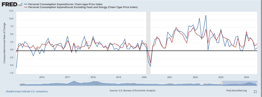
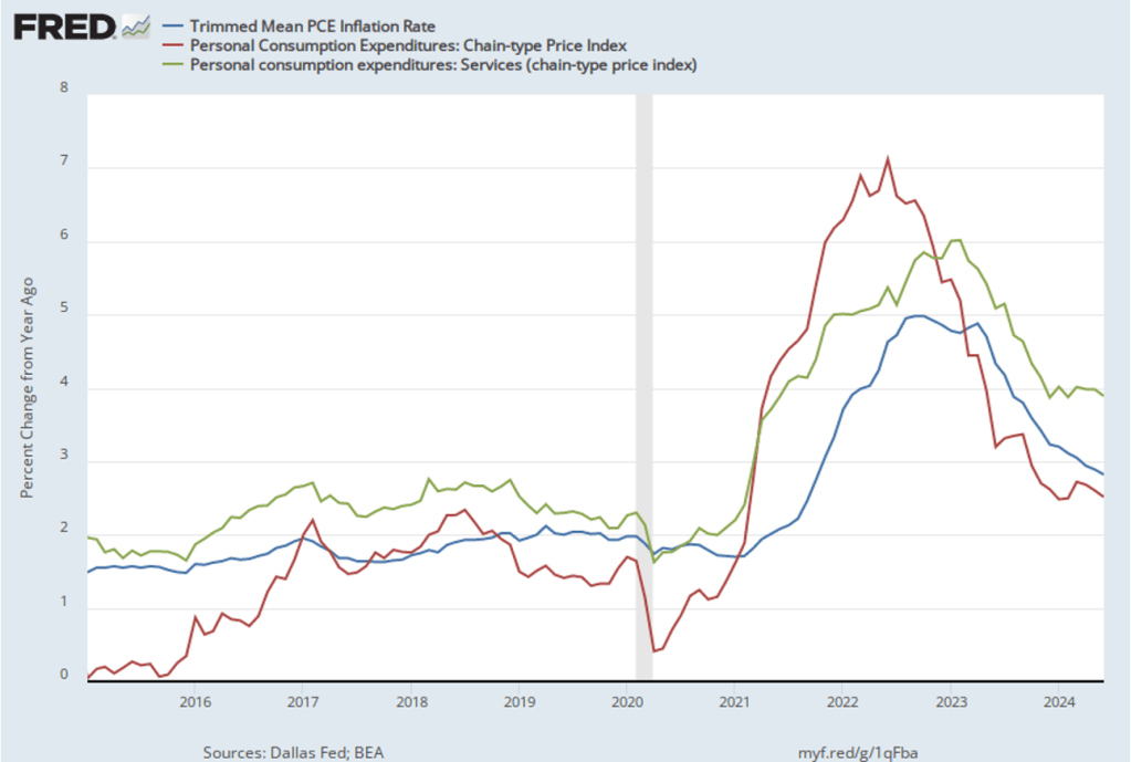
The following figure shows another way of gauging inflation by including the 12-month inflation rate in the PCE (the same as shown in the figure above—although note that PCE inflation is now the red line rather than the blue line), inflation as measured using only the prices of the services included in the PCE (the green line), and the trimmed mean rate of PCE inflation (the blue line). Fed Chair Jerome Powell and other members of the Federal Open Market Committee (FOMC) have said that they are concerned by the persistence of elevated rates of inflation in services. The trimmed mean measure is compiled by economists at the Federal Reserve Bank of Dallas by dropping from the PCE the goods and services that have the highest and lowest rates of inflation. It can be thought of as another way of looking at core inflation by excluding the prices of goods and services that had particularly high or particularly low rates of inflation during the month.
Inflation using the trimmed mean measure was 2.8 percent in June (calculated as a 12-month inflation rate), down only slightly from 2.9 percent in May—and still above the Fed’s target inflation rate of 2 percent. Inflation in services remained high in June at 3.9 percent, down only slightly from 4.0 percent in May.
This month’s PCE inflation data indicate that the inflation rate is still declining towards the Fed’s target, with the low 1-month inflation rates being particularly encouraging. It now seems likely that the FOMC will soon lower the committee’s target for the federal funds rate, which is currently 5.25 percent to 5.50 percent. Remarks by Fed Chair Powell have been interpreted as hinting as much. The next meeting of the FOMC is July 30-31. What do financial markets think the FOMC will decide at that meeting?
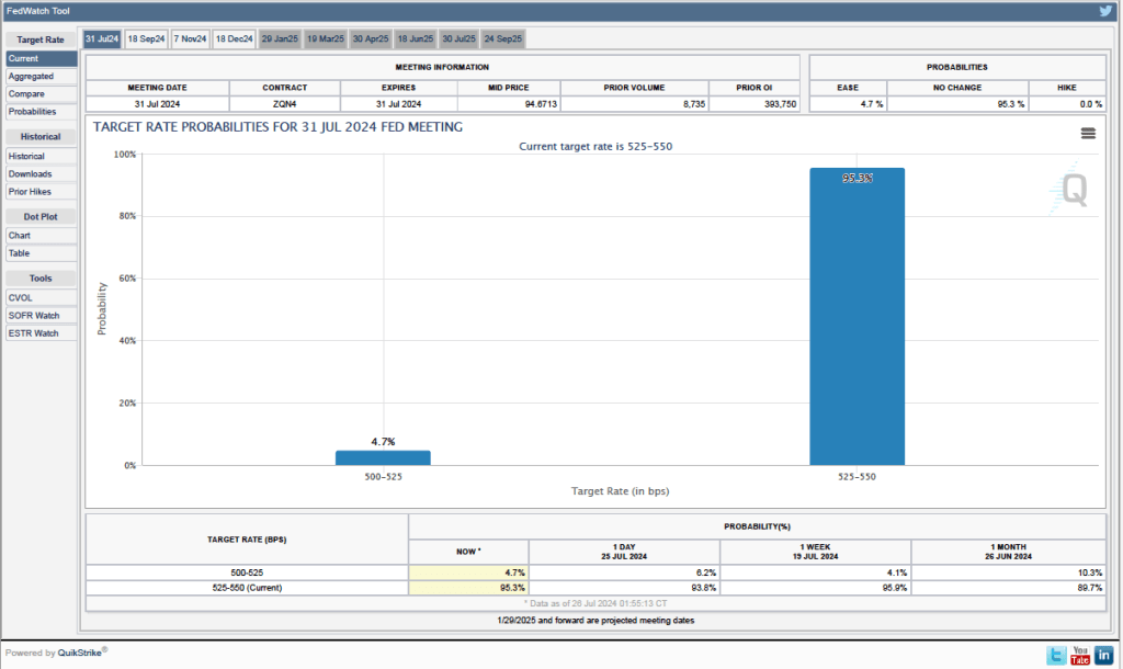
Futures markets allow investors to buy and sell futures contracts on commodities–such as wheat and oil–and on financial assets. Investors can use futures contracts both to hedge against risk—such as a sudden increase in oil prices or in interest rates—and to speculate by, in effect, betting on whether the price of a commodity or financial asset is likely to rise or fall. (We discuss the mechanics of futures markets in Chapter 7, Section 7.3 of Money, Banking, and the Financial System.) The CME Group was formed from several futures markets, including the Chicago Mercantile Exchange, and allows investors to trade federal funds futures contracts. The data that result from trading on the CME indicate what investors in financial markets expect future values of the federal funds rate to be. The following chart from the CME’s FedWatch Tool shows the current values from trading of federal funds futures.
The probabilities in the chart reflect investors’ predictions of what the FOMC’s target for the federal funds rate will be after the committee’s July meeting. The chart indicates that investors assign a probability of only 4.7 percent to the FOMC cutting its federal funds rate target by 0.25 percentage point at its July 30-31 meeting and an 95.3 percent probability of the commitee leaving the target unchanged.
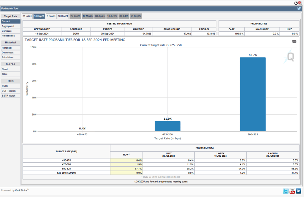
In contrast, the following figure shows that investors expect that the FOMC will cut its federal funds rate at the meeting scheduled for September 17-18. Investors assign an 87.7 percent probability of a 0.25 percentage point cut and a 11.9 percent probability of a 0.50 percentage point cut. The committee deciding to leave the target unchanged at 5.25 percent to 5.50 percent is effectively assigned a zero probability. In other words, investors believe with near certainty that the FOMC will reduce its target for the federal funds rate for the first time since the current round of rate increases ended in July 2023.
Ninteenth century populist William Jennings Bryan delivering a campaign speech. (Photo from the AP via politico.com)
The following op-ed originally appeared in the Wall Street Journal.
The Economic Populists Have a Point
Many issues divide voters heading into the November election, but the economy may be the most crucial. Sound economic policy can foster prosperity and high living standards and affect income and opportunities. Economic resources can also enable society to fund defense or address social and environmental concerns.
Conservative economic policy traditionally has emphasized the openness of markets and growth. By contrast, the populist conservative ideas under discussion at the Republican National Convention focus on people and places hard hit by the disruption that accompanies openness and growth. While many commentators emphasize the differences between the two approaches, a modern conservative economic agenda should build on elements of both.
To begin, a conservative economic agenda should include policies that advance economic growth and living standards. That means supporting research and development, maintaining pro-investment business tax provisions in the Tax Cuts and Jobs Act of 2017, and making regulations that benefit everyone. Such an economy lets businesses and individuals get the most out of the opportunities they seize.
Populist conservatives argue that this traditional approach to policy misses an important objective: a disruptive, rough-and-tumble economy, guided by technological advances and globalization, one that brings everyone along. Populist conservatives want more emphasis on protecting jobs and communities.
There’s more to the populist conservatives’ skepticism than traditional conservatives acknowledge. But backward-looking protectionist measures such as inflationary tariffs or industrial policy aren’t the answer.
However, there is a conservative economic agenda that can unite these groups. The shortcomings of Bidenomics give conservatives an opening to push beyond both market-only neoliberalism and the statist tendencies of industrial policy and protectionism, with their attendant economic inefficiencies. To do so, conservative economic policy needs three ingredients.
The first is agreeing with populist conservatives that markets don’t always work perfectly and that a hands-off approach isn’t always the solution. The state can play a useful role in the market economy. Supply-chain restrictions and export controls can be tools to deny national-security-sensitive technologies to adversaries such as China. But an economic agenda requires more than a sound bite to avoid overreach—such as using “national security” as a pretext for slapping steel tariffs on Canada.
The second essential is competition—the linchpin of economic possibilities for classical economic thinkers from Adam Smith onward. While competition at home and abroad expands the economic pie, it says little about the relative sizes of the slices, a point noted by populist conservatives. A modern conservative economic approach would not only promote competition but also prepare more individuals to compete in a changing economy. One avenue could be supporting community colleges that understand local job needs rather than establishing more government training programs.
Third and most important, a conservative economic platform should recall why conservatives have stressed the benefits of markets. The goal, as my Columbia colleague and Nobel laureate Edmund Phelps puts it, is “mass flourishing.” That is why we want markets to work—to advance innovation and productivity and allow communities to make that flourishing possible.
As far as government’s role, a contemporary economic agenda should recognize a limited measure of successful industrial policy. Two roads should be on offer. The first is to provide more general support for basic and applied research, while letting market forces determine winners and losers. The second is to assign specific goals to particular interventions. The Apollo program’s goal was to put a man on the moon in a decade. The Trump administration’s Operation Warp Speed sought vaccines against Covid.
Populist conservatives are right that there is a role in a conservative economic agenda for helping areas hard hit by disruption. But that role isn’t a mercantilist blunderbuss of protectionism and industrial policy to turn back the economic clock. Rather, place-based aid could support business services for firms trying to create local jobs.
The economic ideas under discussion at the Republican National Convention have populist features that haven’t figured in earlier conservative economic agendas. Populists have some reasonable skepticism about excessive deference to markets. But avoiding excessive meddling from tempting protectionism and the mushy mercantilism of Bidenomics is important, too. Under a conservative economic agenda, growth can flourish.
Chicago Cubs Hall of Fame shortstop Ernie Banks was known for saying “It’s a great day for baseball. Let’s play two!” (Photo from the Baseball Hall of Fame)
First Solved Problem: Exchange Rates and Tourism
Supports: Macroeconomics, Chapter 18, Sections 18.2 and 18.6; and Economics, Chapter 28, Sections 28.2 and 28.6.
The headline of an article on nbcnews.com is: “The Fed May Soon Cut Interest Rates. That Could Make Your Next Trip Abroad More Expensive.”
Briefly explain the difference between a “strong dollar” and a “weak dollar.”
If you are going to spend two weeks on vacation in France, would you prefer that the dollar be strong or weak during that time? Briefly explain.
Briefly explain the connection between Federal Reserve monetary policy and the exchange rate between the U.S. dollar and other currencies.
Use your answers to parts a., b., and c. to explain what the headline means.
Solving the Problem
Step 1: Review the chapter material. This problem is about the effect of changes in exchange rates on import and export prices and the effect of changes in interest rates on exchange rates, so you may want to review Chapter 18, Sections 18.2 and 18.6.
Step 2: Answer part a. by explaining the difference between a “strong dollar” and a “weak dollar.” Generally, the U.S. dollar is called strong when it exchanges for more units of foreign currencies and is called weak when it exchanges for fewer units of foreign currencies. (Economists are less likely to use the phrases “strong dollar” and “weak dollar” than are members of the media.)
Step 3: Answer part b. by expalining whether you would like the U.S. dollar to be weak or strong during your vacation in France. France uses the euro as its currency. As a tourist, you will buy goods and services—such as restaurant meals and souvenirs—in euros. You would like the dollar to be strong because then you will be able to use fewer dollars to exhange for the euros you need to buy goods and services during your vacation.
Step 4: Answer part c. by explaining how Federal Reserve monetary policy affects the exchange rate. As we discuss in Section 18.6, when the Fed wants to pursue an expansionary monetary policy, the Federal Open Market Committee (FOMC) reduces its target for the federal funds rate, which typically results in other interest rates also declining. Lower interest rates make U.S. financial asses, such as Treasury bonds, less attractive relative to foreign financial assets, such as bonds issued by the French government. As a result the demand for U.S. dollars falls relative to the demand for foreign currencies, reducing the exchange rate between the dollar and other currencies. In other words, an expansionary monetary policy will result in a weaker dollar.
Step 5: Answer part d. by using your answers to parts a., b., and c. to expalin what the headline means. The headline indicates that the Fed may soon engage in an expansionary monetary policy, which will result in lower interest rates in the United States, leading to a weaker U.S. dollar. The weaker the dollar, the more dollars you will have to exchange to receive the same number of units of a foreign currency, causing you to have to spend more dollars to pay for the same goods and services during your trip. So, the Fed taking action to reduce interest rates will make your trip abroad more expensive.
Second Solved Problem: Solved Problem: Javier Milei and Argentina’s Exchange Rate Policy
Supports: Macroeconomics, Chapter 18, Sections 18.2 and 18.3; and Economics, Chapter 28, Sections 28.2 and 28.3.
Javier Milei was elected president of Argentina in December 2023. During the presidential campaign he proposed using market-based policies to address Argentina’s economic problems, particularly high rates of inflation and low rates of economic growth. One part of his program involves moving the government away from controlling the value of the peso either by allowing it to float or by making the U.S. dollar legal tender in Argentina. Initially, however, although Milei devalued the peso against the dollar, he didn’t allow the peso to float, keeping the peso pegged against the value of the dollar. An article in the Economist states that many economists believe that the peso is overvalued. The article notes that: “A pricey peso scares off tourists, makes exports expensive and deters investors.” The article also notes that allowing the peso to float “would probably push up inflation.”
Briefly explain what it means for a government to allow its currency to float.
What does it mean to say that a county’s currency is overvalued?
What does the article mean by a “pricey peso”? Why would a pricey peso scare off tourists, make exports expensive, and deter investors?
Why would allowing the peso to float probably push up inflation?
Solving the Problem
Step 1: Review the chapter material. This problem is about exchange rates and exchange rate systems, so you may want to review Chapter 18, Sections 18.2 18.3.
Step 2: Answer part a. by explaining what it means for a government to allow its currency to float. As we discuss in Section 18.3, when a government allows its currency to float it allows the exchange rate between its currency and other currencies to be determined by demand and supply in foreign exchange markets.
Step 3: Answer part b. by expalining what it means for a country’s currency to be overvalued. A currency is overvalued if a government pegs the exchange rate above the market equilibrium exchange rate.
Step 4: Answer part c. by explaining what a “pricey peso” means and why a pricey peso might scare off tourists, make exports expensive, and deter investors. In the context of this article, a pricey peso means an overvalued peso—one that is pegged above the market equilibrium exchange rate, as we noted in the answer to part b. If the peso is overvalued relative to other currencies, then tourists from those countries will find the prices of goods and services in Argentina to be high relative to the prices of those goods and services priced in their domestic currencies. We would expect that fewer foreing tourists would visit Argentina. A pricey peso would make the prices of Argentine exports higher in terms of U.S. dollars, euros, and other currencies. Those high prices will cause a decline in Argentine exports. Finally, a pricey peso will also discourage foreign investors from investing in Argentina because they will receive fewer units of their domestic currency in exchange for the pesos they earn from their investments in Argentina.
Step 5: Answer part d. by explaining why the Argentine government allowing the peso to float would likely increase inflation. The Argentine peso is overvalued, so allowing it to float will cause the value of the peso to decline relative to other currencies. As a result, the peso price of imports will increase. The prices of imported goods and services are included in the price indexes used to measure inflation, so floating the peso will likely increase the inflation rate in Argentina.
Image of servers in a restaurant generated by ChatGTP-4o.
How should you track over time the real wagees of low-wage workers? If you are interested in income mobility, you would want to track the experience over the course of their working lives of individuals who began their careers in low-wage occupations. Doing so would allow you to measure how well (or poorly) the U.S. economy succeeds in providing individuals with opportunities to improve their incomes over time.
You might also be interested in how the real wages of people who earn low wages has changed over time. In this case, rather than tracing the wages over time of individuals who earn low wages when they first enter the labor market, you would look at the real wages of people who earn low wages at any given time. The simplest way to do that analysis would be using data on the average nominal wage earned by, say, the lowest 20 percent of wage earners, and deflate the average nominal wage by a price index to determine the average real wage of these workers. How the average real wage of low-wage workers varies over time provides some insight into the changing standard of living of low-wage workers.
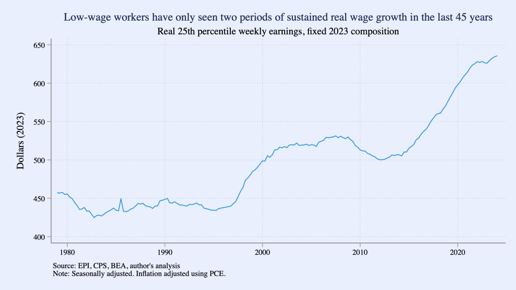
In a recent Substack post, Ernie Tedeschi, Director of Economics at the Budget Lab research center at Yale University, has carried out a careful analysis of movements over time in the average real wage of low-wage workers. Tedeschi points out a complicating factor in this analysis: “The population has gotten older over time and more educated. The workforce looks different too, with more workers in services and fewer in manufacturing. Shifting populations means that comparisons of workers aren’t apples-to-apples over time.”
To correct for these confounding factors, Tedeschi constructs a low-wage index that makes it possible to examine the real wage of low-wage workers, holding constant the composition of low-wage workers with respect to “sex, age, race, college education, and broad industry and occupation” at the values of these characteristics in 2023. Using this approach, makes it possible to separate changes in wages of workers with given characteristics from changes in wages that occur because the average characteristics of workers has changed. For example, on average, workers who are older or who have more years of education will be more productive and, therefore, on average will earn higher wages than will workers who are younger or have fewer years of education.
The following figure from Tedeschi’sSubstack post shows movements in his low-wage index during each quarter from the first quarter of 1979 to the first quarter of 2024, with “low wage” defined as workers at the 25th precentile of the distribution of wages. (That is, 24 percent of workers receive lower wages and 75 percent of workers receive higher wages than do these workers.) The index shows that a low-wage worker in 2024 has a much higher real wage than a low-wage worker in 1979, but the increase in the average real wage occurs mainly during two periods: 1997–2007 and 2014–2024. (Tedeschi uses the person consumption expenditures (PCE) price index to convert nominal wages to real wages.)
A more complete discussion of Tedeschi’s methods and results can be found in his blog post.
Jerome Powell arriving to testify before Congress. (Photo from Bloomberg News via the Wall Street Journal.)
Each month the Bureau of Labor Statistics (BLS) releases its “Employment Situation” report. As we’ve discussed in previous blog posts, discussions of the report in the media, on Wall Street, and among policymakers center on the estimate of the net increase in employment that the BLS calculates from the establishment survey.
How should the members of the Fed’s policy-making Federal Open Market Committee interpret these data? For instance, the BLS reported that the net increases in employment in June was 206,000. (Always worth bearing in mind that the monthly data are subject to—sometimes substantial—revisions.) Does a net increase of employment of that size indicate that the labor market is still running hot—with the quantity of labor demanded by businesses being greater than the quantity of labor workers are supplying—or that the market is becoming balanced with the quantity of labor demanded roughly equal to the quantity of labor supplied?
On July 9, in testimony before the Senate Banking Committee indicated that his interpretation of labor market data indicate that: “The labor market appears to be fully back in balance.” One interpretation of the labor market being in balance is that the number of net new jobs the economy creates is enough to keep up with population growth. In recent years, that number has been estimated to be 70,000 to 100,000. The number is difficult to estimate with precision for two main reasons:
There is some uncertainty about the number of older workers who will retire. The more workers who retire, the fewer net new jobs the economy needs to create to accommodate population growth.
More importantly, estimates of population growth are uncertain, largely because of disagreements among economists and demographers over the number of immigrants who have entered the United States in recent years.
In calculating the unemployment rate and the size of the labor force, the BLS relies on estimates of population from the Census Bureau. In a January report, the Congressional Budget Office (CBO) argued that the Census Bureau’s estimate of the population of the United States is too low by about 6 million people. As the following figure from the CBO report indicates, the CBO believes that the Census Bureau has underestimated how much immigration has occurred and what the level of immigration is likely to be over the next few years. (In the figure, SSA refers to the Social Security Administration, which also makes forecasts of population growth.)
Some economists and policymakers have been surprised that low levels of unemployment and large monthly increases in employment have not resulted in greater upward pressure on wages. If the CBO’s estimates are correct, the supply of labor has been increasing more rapidly than is indicated by census data, which may account for the relative lack of upward pressure on wages. If the CBO’s estimates of population growth are correct, a net increase in employment of 200,000, as occured in June, may be about the number necessary to accommodate growth in the labor force. In other words, Chair Powell would be correct that the labor market was in balance in June.
In a recent publication, economists Nicolas Petrosky-Nadeau and Stephanie A. Stewart of the Federal Reserve Bank of San Francisco look at a related concept: breakeven employment growth—the rate of employment growth required to keep the unemployment rate unchanged. They estimate that high rates of immigration during the past few years have raised the rate of breakeven employment growth from 70,000 to 90,000 jobs per month to 230,000 jobs per month. This analysis would be consistent with the fact that as net employment increases have averaged 177,000 over the past three months—somewhat below their estimate of breakeven employment growth—the unemployment rate has increased from 3.8 percent to 4.1 percent.
Image of “a family shopping in a supermarket” generated by ChatGTP 4o.
In testifying before Congress this week, Federal Reserve Chair Jerome Powell indicated that the Fed’s policy-making Federal Open Market Committee (FOMC) was becoming more concerned that it not be too late in reducing its target for the federal funds rate:
“[I]n light of the progress made both in lowering inflation and in cooling the labor market over the past two years, elevated inflation is not the only risk we face. Reducing policy restraint too late or too little could unduly weaken economic activity and employment.”
Powell also noted that: “more good data would strengthen our confidence that inflation is moving sustainably toward 2 percent.” Today (July 11), Powell received more good data as the Bureau of Labor Statistics (BLS) released its monthly report on the consumer price index (CPI), which showed a further slowing in inflation.
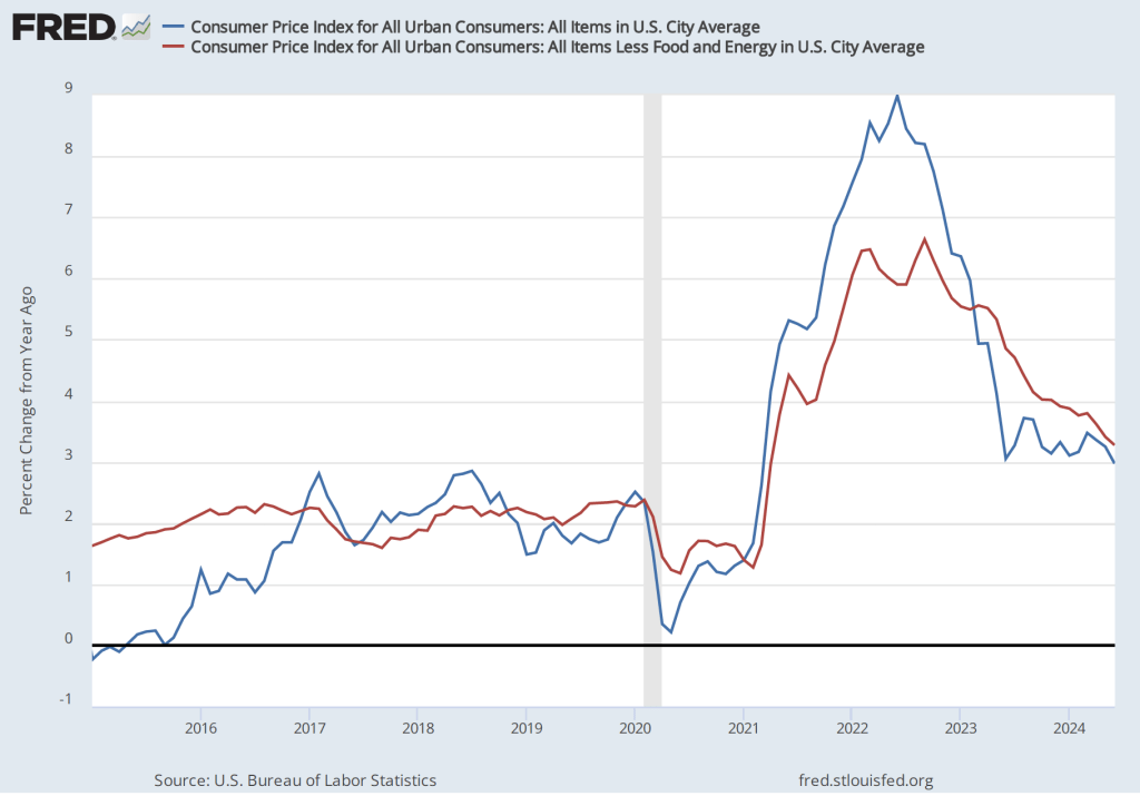
As the following figure shows, the inflation rate for June measured by the percentage change in the CPI from the same month in the previous month—headline inflation (the blue line)—was 3.o percent down from 3.3 percent in May. Core inflation (the red line)—which excludes the prices of food and energy—was 3.3 percent in June, down from 3.4 percent in May.
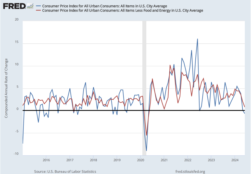
As the following figure shows, if we look at the 1-month inflation rate for headline and core inflation—that is the annual inflation rate calculated by compounding the current month’s rate over an entire year—the declines in the inflation rate are much larger. Headline inflation (the blue line) declined from 0.1 percent in May to –0.7 in June—consumer prices fell during June. Core inflation (the red line) declined from 2.0 percent in May to 0.8 percent in June. Overall, we can say that inflation has cooled further in June, bringing the U.S. economy closer to a soft landing—with the annual inflation rate returning to the Fed’s 2 percent target without the economy being pushed into a recession. (Note, though, that the Fed uses the personal consumption expenditures (PCE) price index, rather than the CPI in evaluating whether it is hitting its 2 percent inflation target.)
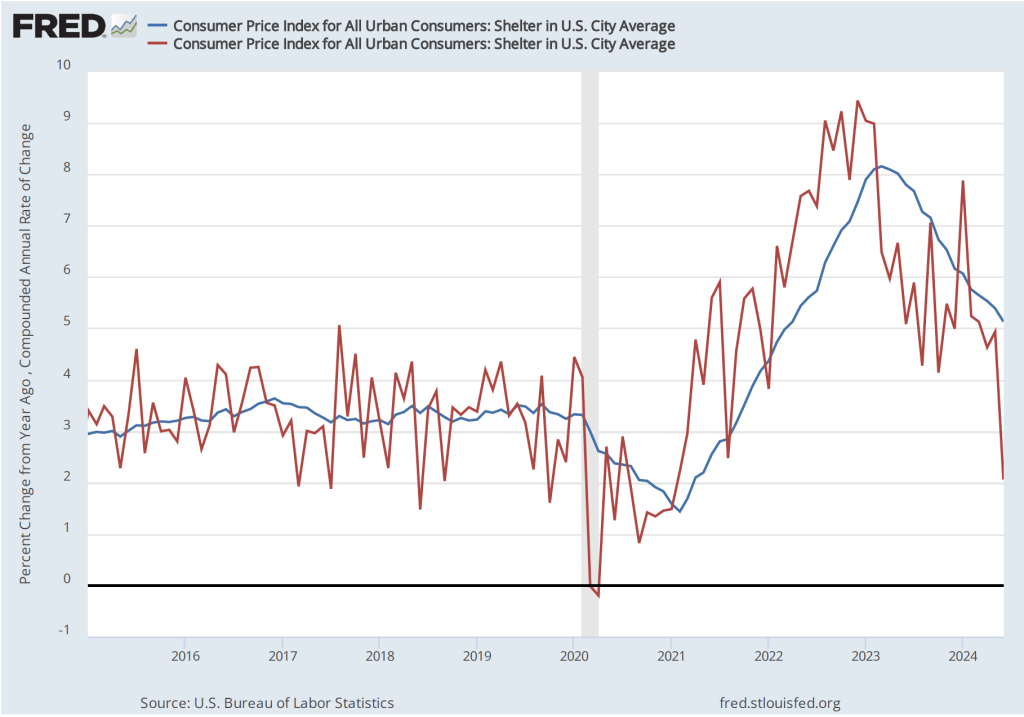
The FOMC has been looking closely at inflation in the price of shelter. The price of “shelter” in the CPI, as explained here, includes both rent paid for an apartment or house and “owners’ equivalent rent of residences (OER),” which is an estimate of what a house (or apartment) would rent for if the owner were renting it out. OER is included to account for the value of the services an owner receives from living in an apartment or house.
As the following figure shows, inflation in the price of shelter has been a significant contributor to headline inflation. The blue line shows 12-month inflation in shelter and the red line shows 1-month inflation in shelter. Twelve-month inflation in shelter continued its decline that began in the spring of 2023. One-month inflation in shelter declined substantially from 4.9 percent in May to 2.1 percent in June. These values indicate that the price of shelter may no longer be a significant driver of headline inflation.
Finally, in order to get a better estimate of the underlying trend in inflation, some economists look at median inflation and trimmed mean inflation. Meadin inflation is calculated by economists at the Federal Reserve Bank of Cleveland and Ohio State University. If we listed the inflation rate in each individual good or service in the CPI, median inflation is the inflation rate of the good or service that is in the middle of the list—that is, the inflation rate in the price of the good or service that has an equal number of higher and lower inflation rates. Trimmed mean inflation drops the 8 percent of good and services with the higherst inflation rates and the 8 percent of goods and services with the lowest inflation rates.
As the following figure (from the Federal Reserve Bank of Cleveland) shows, both median inflation (the brown line) and trimmed mean inflation (the blue line) were somewhat higher than either headline CPI inflation or core CPI inflation. One conclusion from these data is that headline and core inflation may be somewhat understating the underlying rate of inflation.
Financial markets are interpreting the most inflation and employment data as indicating that at its meeting on Septembe 17-18 the FOMC is likely to cut its target range for the federal funds rate from the current 5.25 percent to 5.50 to 5.00 percent to 5.25 percent.
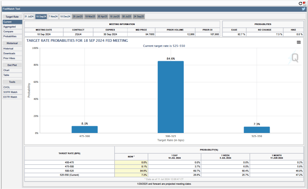
Futures markets allow investors to buy and sell futures contracts on commodities–such as wheat and oil–and on financial assets. Investors can use futures contracts both to hedge against risk—such as a sudden increase in oil prices or in interest rates—and to speculate by, in effect, betting on whether the price of a commodity or financial asset is likely to rise or fall. (We discuss the mechanics of futures markets in Chapter 7, Section 7.3 of Money, Banking, and the Financial System.) The CME Group was formed from several futures markets, including the Chicago Mercantile Exchange, and allows investors to trade federal funds futures contracts. The data that result from trading on the CME indicate what investors in financial markets expect future values of the federal funds rate to be. The following chart from the CME’s FedWatch Tool shows the current values from trading of federal funds futures.
The probabilities in the chart reflect investors’ predictions of what the FOMC’s target for the federal funds rate will be after the committee’s September meeting. The chart indicates that investors assign a probability of only 8.1 percent to the FOMC leaving its federal funds rate target unchanged at its September meeting, but a 84.6 percent probability of the committee cutting its target by 0.25 percentage point (and a 7.3 percent probability of the committee cutting its target by 0.50 percent age point).
Recent macroeconomic data have been sending mixed signals about the state of the U.S. economy. The growth in real GDP, industrial production, retail sales, and real consumption spending has been slowing. Growth in employment has been a bright spot—showing steady net increases in job growth above the level necessary to keep up with population growth. Even here, though, as we discuss in a recent blog post, the data may be overstating the actual strength of the labor market.
This morning (July 5), the Bureau of Labor Statistics (BLS) released its “Employment Situation” report (often referred to as the “jobs report”) for June, which, while seemingly indicating continued strong job growth, also provides some indications that the labor market may be weakening. The jobs report has two estimates of the change in employment during the month: one estimate from the establishment survey, often referred to as the payroll survey, and one from the household survey. As we discuss in Macroeconomics, Chapter 9, Section 9.1 (Economics, Chapter 19, Section 19.1), many economists and policymakers at the Federal Reserve believe that employment data from the establishment survey provides a more accurate indicator of the state of the labor market than do either the employment data or the unemployment data from the household survey. (The groups included in the employment estimates from the two surveys are somewhat different, as we discuss in this post.)
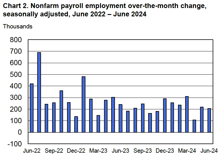
According to the establishment survey, there was a net increase of 206,000 jobs during April. This increase was a little above the increase of 1900,000 to 200,000 that economists had forecast in surveys by the Wall Street Journal and bloomberg.com. The following figure, taken from the BLS report, shows the monthly net changes in employment for each month during the past to years.
It’s notable that the previously reported increases in employment for April and May were revised downward by 110,000 jobs, or by about 25 percent. (The BLS notes that: “Monthly revisions result from additional reports received from businesses and government agencies since the last published estimates and from the recalculation of seasonal factors.”) As we’ve discussed in previous posts (most recently here), revisions to the payroll employment estimates can be particularly large at the beginning of a recession.
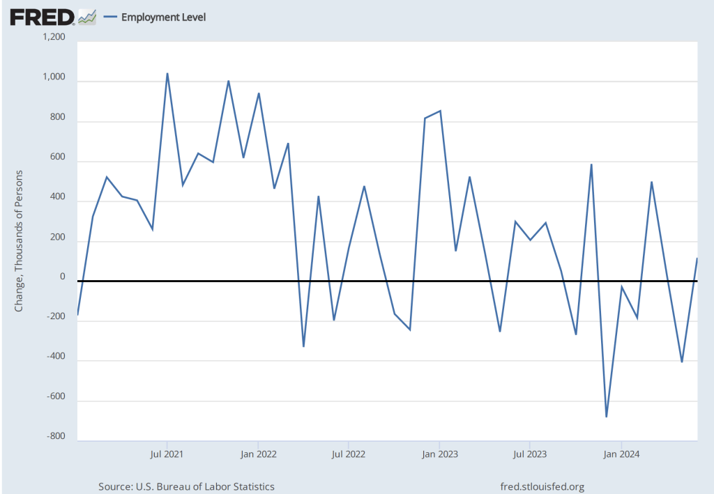
As the following figure shows, the net change in jobs from the household survey moves much more erratically than does the net change in jobs in the establishment survey. The net increase in jobs as measured by the household survey increased from –408,000 in May (that is, employment by this measure fell during May) to 116,000 in June.
Note that the BLS also reports a survey for household employment adjusted to conform to the concepts and definitions used to construct the payroll employment series. After this adjustment, over the past 12 months household employment has increased by 32.5 million less than has payroll employment. Clearly, this is a very large discrepancy and may be indicating that the payroll survey is substantially overstating growth in employment.
The unemployment rate, which is also reported in the household survey, ticked up slightly from 4.0 percent to 4.1 percent. Although still low by historical standards, June was the fourth consecutive month in which the unemployment rate increased.
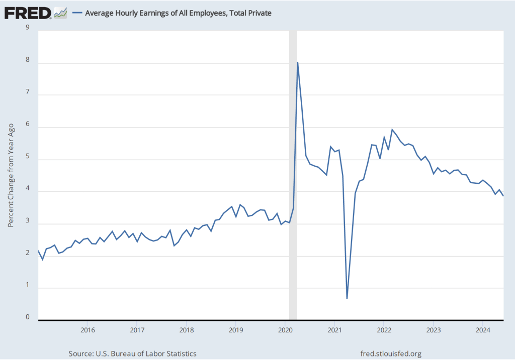
The establishment survey also includes data on average hourly earnings (AHE). As we note in this post, many economists and policymakers believe the employment cost index (ECI) is a better measure of wage pressures in the economy than is the AHE. The AHE does have the important advantage that it is available monthly, whereas the ECI is only available quarterly. The following figure show the percentage change in the AHE from the same month in the previous year. The 3.9 percent increase for June continues a downward trend that began in January and is the smallest increase since June 2021.
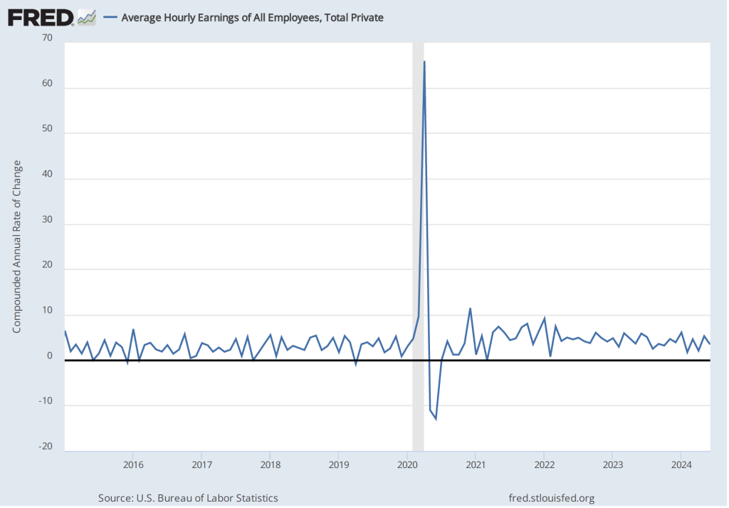
The following figure shows wage inflation calculated by compounding the current month’s rate over an entire year. (The figure above shows what is sometimes called 12-month wage inflation, whereas this figure shows 1-month wage inflation.) One-month wage inflation is much more volatile than 12-month inflation—note the very large swings in 1-month wage inflation in April and May 2020 during the business closures caused by the Covid pandemic.
The 1-month rate of wage inflation of 3.5 percent in June is a significant decrease from the 5.3 percent rate in May, although it’s unclear whether the decline was an additional sign that the labor market is weakening or reflected the greater volatility in wage inflation when calculated this way.
What effect is today’s job reports likely to have on the Fed’s policy-making Federal Open Market Committee as it considers changes in its target for the federal funds rate? As always, it’s a good idea not to rely too heavily on a single data point—particularly because, as we noted earlier, the establishment survey employment data is subject to substantial revisions. But the Wall Street Journal’sheadline that the “Case for September Rate Cut Builds After Slower Jobs Data,” seems likely to be accurate.