Please listen to a podcast discussion recorded just this past Friday between Glenn Hubbard and Tony O’Brien as they discuss tariffs and it’s impact on monetary policy. Also, check out the regular blog posts while on the site! So much has been happening and these posts helps both instructors and students integrate this discussion into their classroom.
Join authors Glenn Hubbard and Tony O’Brien as they discuss the impact of new tariff policies on trade but also on the larger economy. They delve into the Fed, monetary policy, and the impact on inflation. They also discuss some of the history back to when tariffs used to be a high proportion of government revenue and analyze the mix of products that are imported & exported by the US. Should the Fed change its current behavior due to the tariff environment?
Even though Russia and Ukraine were engaged in cease-fire talks with American representatives in Saudi Arabia, apparently with some progress on Tuesday, President Vladimir Putin of Russia has shown little actual commitment to ending his war.
President Trump needs some better cards.
Several weeks ago, the president floated the idea of sanctions and tariffs over Russian imports. But the Kremlin has been dismissive — mainly because the United States imports very little from Russia. Extensive financial and trade sanctions have been in place, most of them for around three years, and they are plainly not enough to bring peace.
Fortunately, there is a simple way to improve the American hand. The administration should impose sanctions on any company or individual — in any country — involved in a Russian oil and gas sale. Russia could avoid these so-called secondary sanctions by paying a per shipment fee to the United States Treasury. The payment would be called a Russian universal tariff, and it would start low but increase every week that passes without a peace deal.
Ships carry most Russian oil and gas to world markets. The secondary sanctions — if Russia does not make the required payments — would fall on all parties to the transaction, including the oil tanker owner, the insurer and the purchaser. Recent evidence confirms that Indian and Chinese entities — whose nations import considerable oil from Russia and have not imposed their own penalties on the Russian economy over the war in Ukraine — do not want to be caught up in American sanctions, making this idea workable. Another factor in its favor: All such tanker traffic is tracked carefully by commercial parties and by U.S. authorities.
Secondary sanctions are powerful tools: Violators can be cut off from the U.S. financial system, and they apply even to transactions that don’t directly involve American companies. They have been used to limit Iranian oil exports and to require that payments for Iranian oil be held in restricted accounts until sanctions were lifted. Our proposal would take this approach to another level. Under our plan, a portion of each Russian oil and gas sale would be paid to the U.S. Treasury until Russia agrees to a peace deal. The goal is to keep Russian oil flowing to global markets but with less money going to the Kremlin. The plan would sap Russia’s ability to continue waging war, and it puts money into U.S. government coffers.
In Russia, fossil fuel revenues and military spending are intertwined, although the country can also draw on its sovereign wealth fund and other sources. Fossil fuel exports provide the main source of dollar revenue for the Kremlin, which depends on hard currency to buy arms and other military supplies from abroad and pay for North Korean soldiers. The country currently exports about $500 million worth of crude oil and petroleum products and $100 million worth of natural gas every day. The Kremlin budgeted a slightly lower amount, almost $400 million per day for military spending in 2025.
The Russia universal tariff would provide money for the United States immediately, unlike the proposed Ukrainian critical minerals fund, which would take years to generate any returns. A fee of $20 per barrel of oil could generate up to $120 million per day (more than $40 billion per year), with additional revenue available if a similar fee is imposed on natural gas. Every dollar the United States collects is a dollar that Russia can’t spend to fund its war.
Ideally, the policy would pressure Russia into negotiations, where its removal could be part of a deal. If not, the United States would still collect billions annually, which could help fund Mr. Trump’s proposed tax cuts. In that scenario, Russia would effectively be helping repaythe U.S. tax dollars used to provide aid to Ukraine to defend itself against Russia’s assault.
For the past three years, Western sanctions and public outcry, including some dockworkers’ refusal to unload Russian oil tankers, have forced Russia to search for new buyers and sell its oil at a discount compared with global prices. The oil discount averaged about $9 per barrel over the previous 12 months and was as high as $35 per barrel in April 2022. Despite receiving lower prices for its oil, Russia has maintained export volumes, ensuring a steady supply in the global oil market.
By imposing secondary sanctions unless the Russia universal tariff is paid, the United States would be taking a cut of the revenues, effectively increasing the discount on Russian oil. Russia’s continued exports, despite facing large discounts over the past three years, suggest it would continue exporting the same volume. That would keep global oil supply stable and help keep oil prices in check. Oil and gas in Russia are inexpensive to produce, and it relies heavily on the income they generate, so it has little option but to keep selling, even at lower prices.
While Mr. Trump can adopt this strategy, Congress can strengthen his negotiating position by passing a bill that puts the Russia universal tariff in place on its own. That would allow the president to protect his lines of communication with Mr. Putin by blaming the measure on Congress. He would also determine if and when he wants to sign the bill, giving him additional leverage over Russia. It’s possible the mere discussion of such a bill could help push the Kremlin toward a peace deal.
Combining secondary sanctions, a strong tool in the U.S. economic kit, with a tarifflike fee could pressure Mr. Putin by threatening his most valuable source of revenues. It would also make it easier for Mr. Trump to deliver on his promise of a lasting peace.
Catherine Wolfram, a former deputy assistant secretary for climate and energy in the Treasury Department, is a professor at M.I.T.’s Sloan School of Management.
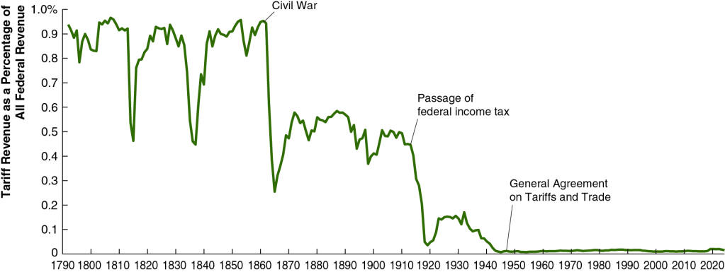
A tariff is a tax a government imposes on imports. Since the end of World War II, high-income countries have only occasionally used tariffs as an important policy tool. The following figure shows how the average U.S. tariff rate, expressed as a percentage of the value of total imports, has changed in the years since 1790. The ups and downs in tariff rates reflect in part political disa-greements in Congress. Generally speaking, through the early twentieth century, members of Congress who represented areas in the Midwest and Northeast that were home to many manufacturing firms favored high tariffs to protect those industries from foreign competition. Members of Congress from rural areas opposed tariffs, because farmers were primarily exporters who feared that foreign governments would respond to U.S. tariffs by imposing tariffs on U.S. agricultural exports. From the pre-Civil War period until after World War II the Republicans Party generally favored high tariffs and the Democratic Party generally favored low tariffs, reflecting the economic interests of the areas the parties represented in Congress. (Note: Because the tariffs that the Trump Administration will end up imposing are still in flux, the value for 2025 in the figure is only a rough estimate.)
By the end of World War II in 1945, government officials in the United States and Europe were looking for a way to reduce tariffs and revive international trade. To help achieve this goal, they set up the General Agreement on Tariffs and Trade (GATT) in 1948. Countries that joined the GATT agreed not to impose new tariffs or import quotas. In addition, a series of multilateral negotiations, called trade rounds, took place, in which countries agreed to reduce tariffs from the very high levels of the 1930s. The GATT primarily covered trade in goods. A new agreement to cover services and intellectual property, as well as goods, was eventually negotiated, and in January 1995, the GATT was replaced by the World Trade Organization (WTO). In 2025, 166 countries are members of the WTO.
As a result of U.S. participation in the GATT and WTO, the average U.S. tariff rate declined from nearly 20% in the early 1930s to 1.8% in 2018. The first Trump Administration increased tariffs beginning in 2018, raising the average tariff rate to 2.5%. (The Biden Administration continued most of the increases.) In 2025, the second Trump Administration’s substantial increases in tariffs raised the average tariff rate to the highest level since the 1940s.
Until the enactment in 1913 of the 16th Amendment to the U.S. Constitution, which allowed for a federal income tax, tariffs were an important source of revenue to the federal government. As the following figure shows, in the early years of the United States, more than 90% of federal government revenues came from the tariff. As tariff rates declined and federal income and payroll taxes increased, tariffs declined to only 2% of federal government revenue. It’s unclear yet how much tariff’s share of federal government revenue will rise as a result of the Trump Administration’s tariff increases.
The effect of tariff increases on the U.S. economy are complex and depend on the details of which tariffs are increased, by how much they are increased, and whether foreign governments raise their tariffs on U.S. exports in response to U.S. tariff increases. We can analyze some of the effects of tariffs using the basic aggregate demand and aggregate supply model that we discuss in Macroeconomics, Chapter 13 (Economics, Chapter 23). We need to keep in mind in the following discussion that small increases in tariffs rates—such as those enacted in 2018—will likely have only small effects on the economy given that net exports are only about 3% or U.S. GDP.
An increase in tariffs intended to protect domestic industries can cause the aggregate demand curve to shift to the right if consumers switch spending from imports to domestically produced goods, thereby increasing net exports. But this effect can be partially or wholly offset if trading partners retaliate by increasing tariffs on U.S. exports. When Congress passed the Smoot-Hawley Tariff in 1930, which raised tariff rates to historically high levels, retaliation by U.S. trading partners contributed to a sharp decline in U.S. exports during the early 1930s.
International trade can increase a country’s production and income by allowing a country to specialize in the goods and services in which it has a comparative advantage. Tariffs shift a country’s allocation of labor, capital, and other resources away from producing the goods and services it can produce most efficiently and toward producing goods and services that other countries can produce more efficiently. The result of this misallocation of resources is to reduce the productive capacity of the country, shifting the long-run aggregate supply curve (LRAS) to the left.
Tariffs raise the prices of U.S. imports. This effect can be partially offset because tariffs increase the demand for U.S. dollars relative to trading partners’ currencies, increasing the dollar exchange rate. Because a tariff effectively acts as a tax on imports, like other taxes its incidence—the division of the burden of the tax between sellers and buyers—depends partly on the price elasticity of demand and the price elasticity of supply, which vary across the goods and services on which tariffs are imposed. (We discuss the effects of demand and supply elasticity on the incidence of a tax in Microeconomics, Chapter 17, Section 17.3.)
About two-thirds of U.S. imports are raw materials, intermediate goods, or capital goods, all of which are used as inputs by U.S. firms. For example, many cars assembled in the United States contain imported parts. The popular Ford F-Series pickup trucks are assembled in the United States, but more than two-thirds of the parts are imported from other countries. That fact indicates that the automobile industry is one of many U.S. industries that depend on global supply chains that can be disrupted by tariffs. Because tariffs on imported raw materials, parts and other intermediate goods, and capital goods increase the production costs of U.S. firms, tariffs reduce the quantity of goods these firms will produce at any given price. In terms of the aggregate demand and aggregate supply model , a large unexpected increase in tariffs results in an aggregate supply shock to the economy, shifting the short-run aggregate supply curve (SRAS) to the left.
Our thanks to Fernando Quijano for preparing the two figures.
An image generated by GTP-4o illustrating research.
This opinion column by Glenn appeared in the Financial Times on March 10.
The Trump administration has wisely emphasised raising America’s rate of economic growth. But growth doesn’t just happen. It is the byproduct of innovation both radical (think of the emergence of generative artificial intelligence) and gradual (such as improvements in manufacturing processes or transport). Many economic factors influence innovation, but research and development is key. While this can be privately or publicly funded, the latter can support basic research with spillovers to many companies and applications.
Therein lies the rub: the new administration’s growth agenda is joined by a significant effort to reduce government spending, spearheaded by the so-called Department of Government Efficiency. Some spending restraint can enhance growth by reducing interest rates or reallocating funds towards more investment-oriented activities. But cuts to R&D, as the administration is advocating at the National Institutes of Health (NIH), National Science Foundation (NSF), Department of Energy (DoE) and NASA, are counter-productive. They will limit innovation and growth.
The link between R&D and productivity growth has a long pedigree in economics and has generally been acknowledged by US policymakers. In the mid-1950s, economist Robert Solow made the Nobel Prize-winning conclusion that sustained output growth is not possible without technological progress. Decades later, former World Bank chief economist Paul Romer added another Nobel Prize-winning insight: growth reflected the intentional adoption of new ideas, so could be affected by research incentives.
It is well known that research is undervalued by private companies. Private funders of R&D don’t capture all its benefits. The social returns of R&D are two to four times higher than private returns. These high returns are enabled in the US by federal funding. For example, publicly funded research at the NIH has been found to significantly impact private development of new drugs.
In a comprehensive study, Andrew Fieldhouse and Karel Mertens classify major changes in non-defence R&D funding by the DoE, Nasa, NIH and NSF over the postwar period. They estimate implied returns of as much as 200 per cent — raising US economic output by $2 per dollar of funding. This is substantially higher than recent estimates of returns to private R&D. According to the Congressional Budget Office, the high returns to public funding are more than 10 times that on public investment in infrastructure. With the higher tax revenue generated from additional GDP, an increase in R&D funding more than pays for itself.
In aggregate, productivity gains from federal R&D funding are substantial. Indeed, Fieldhouse and Mertens estimate that government-funded R&D amounts to about one-fifth of productivity growth (measured as output growth less all input growth) in the US since the second world war.
Combined with the high social returns of government-funded R&D, it is essential that policymakers in the current administration acknowledge the risks of underfunding R&D. Spending cuts are clearly harmful to productivity and even budget outcomes.
A shift towards government-financed R&D does not imply that policy in these areas should be beyond review. Some economists have questioned whether current R&D projects take sufficiently high scientific risks, particularly on the ideas of younger scholars. And policymakers can certainly investigate whether indirect cost subsidies to universities and laboratories—in addition to the direct costs of research—are set at the appropriate levels. But, if growth is the objective, the presumption must be that additional public spending on R&D is worthwhile.
Federal support for growth-oriented R&D can extend beyond research grants. Publicly supported applied research centres around the country offer a mechanism to collaborate with local universities and business networks to disseminate ideas to practice. This builds upon the agricultural and manufacturing extension services instituted by 19th-century land-grant colleges that enhanced productivity.
The Trump administration is right to promote growth as a public objective. Spending restraint and fiscal discipline can be growth-enhancing. But all spending is equal. Government-funded R&D is vitally important for innovation and productivity growth. The case is clear.
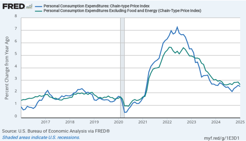
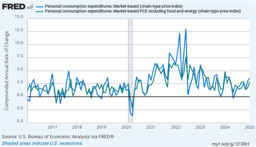
Today (February 28), the BEA released monthly data on the personal consumption expenditures (PCE) price index as part of its “Personal Income and Outlays” report. The Fed relies on annual changes in the PCE price index to evaluate whether it’s meeting its 2 percent annual inflation target. The following figure shows PCE inflation (blue line) and core PCE inflation (green line)—which excludes energy and food prices—for the period since January 2016 with inflation measured as the percentage change in the PCE from the same month in the previous year. Measured this way, in January PCE inflation was 2.5 percent, down slightly from 2.6 in December. Core PCE inflation in January was 2.6 percent, down from 2.9 percent in December. Headline and core PCE inflation were both consistent with the forecasts of economists.
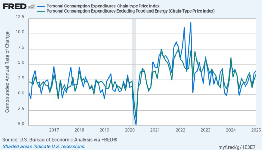
The following figure shows PCE inflation and core PCE inflation calculated by compounding the current month’s rate over an entire year. (The figure above shows what is sometimes called 12-month inflation, while this figure shows 1-month inflation.) Measured this way, PCE inflation rose in January to 4.0 percent from 3.6 percent in December. Core PCE inflation rose in January to 3.5 percent from to 2.5 percent in December. So, both 1-month core PCE inflation estimates are running well above the Fed’s 2 percent target. But the usual caution applies that 1-month inflation figures are volatile (as can be seen in the figure), so we shouldn’t attempt to draw wider conclusions from one month’s data.
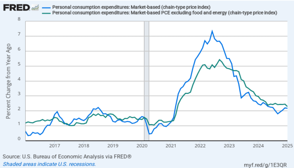
In recent months, Fed Chair Jerome Powell has noted that inflation in non-market services has been high. Non-market services are services whose prices the BEA imputes rather than measures directly. For instance, the BEA assumes that prices of financial services—such as brokerage fees—vary with the prices of financial assets. So that if stock prices rise, the prices of financial services included in the PCE price index also rise. Powell has argued that these imputed prices “don’t really tell us much about … tightness in the economy. They don’t really reflect that.” The following figure shows 12-month headline inflation (the blue line) and 12-month core inflation (the green line) for market-based PCE. (The BEA explains the market-based PCE measure here.)
Headline market-based PCE inflation was 2.2 percent in January, and core market-based PCE inflation was 2.3 percent. So, both market-based measures show less inflation in January than do the total measures. In the following figure, we look at 1-month inflation using these measures. Again, inflation is running somewhat lower when using these market-based measures of inflation. Note, though, that all four market-based measures are running above the Fed’s 2 percent target.
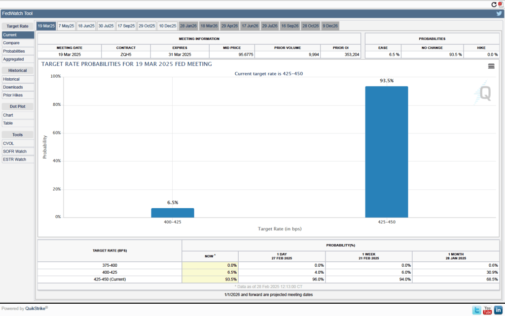
In summary, today’s data don’t change the general picture with respect to inflation: While inflation has substantially declined from its high in mid-2022, it still is running above the Fed’s target of 2 percent. As a result, it’s likely that the Fed’s policymaking Federal Open Market Committee (FOMC) will leave its target for the federal funds rate unchanged at its next meeting on March 18–19.
Investors who buy and sell federal funds futures contracts expect that the FOMC will leave its federal funds rate target unchanged at its next meeting. (We discuss the futures market for federal funds in this blog post.) As the following figure shows, investors assign a probability of 93.5 percent to the FOMC leaving its target for the federal funds rate unchanged at the current range of 4.25 percent to 4.50. Investors assign a probability of only 6.5 percent to the FOMC cutting its target by 0.25 percentage point (25 basis points).
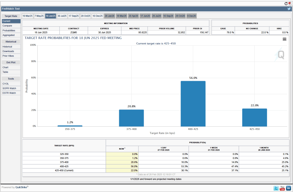
As shown the following figure shows, investors assign a probability of greater than 50 percent that the FOMC will cut its target range by at least 25 basis points at its meeting nearly four months from now on June 17–18. Investors may be concerned that the economy is showing some signs of weakening. Today’s BEA report indicates that real personal consumption expenditures declined at a very high 5.5 percent compound annual rate in January. (Although measured as the 12-month change, real consumption spending increased by 3.o percent in January.)
We’ll have a better understanding of the FOMC’s evaluation of recent macroeconomic data after Chair Powell’s news conference following the March 18–19 meeting.
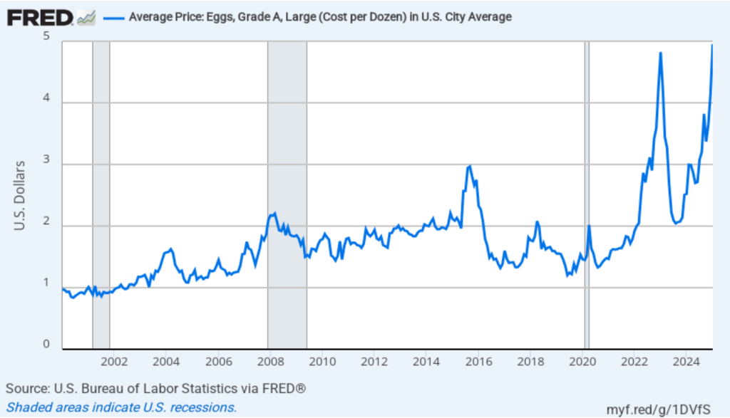
What causes consumer demand for a product to decline? Why does demand for some products suddenly rise? As we discuss in Chapter 3, changes in the relative price of a substitute or a complement cause the demand for a good to shift. For instance, the following figure shows the recent rapid increase in the price of eggs, due in part from the spread of bird flu. We would expect that the increase in the price of eggs will shift to the right the demand curve for egg substitutes, such as the product shown below the figure.
Sometimes a shift in the demand for a product represents a change in consumer tastes. For instance, as we discuss in an Apply the Concept in Chapter 3, for decades most people wore a hat while outdoors. The first photo below shows people walking down a street in New York City in the 1920s. Beginning in the 1960s, hats started to fall out of fashion. As the second photo shows, today few people wear hats—unless they’re walking outside during the winter in the Northeast or the Midwest!
Photo from the New York Daily News
Photo from the New York Times
Technological change can also affect the demand for goods. For example, the development of network television, beginning in the late 1940s, reduced the demand for tickets to movie theaters. Similarly, the development of the internet reduced the demand for physical newspapers.
A recent example of technological change having a substantial effect on a number of consumer goods is the introduction of GLP–1 drugs, beginning in 2005. These drugs, such as Ozempic and Mounjaro, were first developed to treat type 2 diabetes. The drugs were found to significantly reduce appetite in most users, leading to users losing weight. Accordingly, doctors began to prescribe the drugs to treat obesity. By 2025, about half of the users of GLP–1 drugs were doing so to lose weight. A recent article in the Washington Post quoted Jan Hatzius, chief economist at Goldman Sachs, as predicting that by 2028, 60 million people in the United States will be taking a GLP–1 drug.
Many consumers who use these drugs decide to change the mix of foods they eat. Typically, users demand fewer ultra-processed foods, such as chips, cookies, and soft drinks. The percentage of people in the United States who are considered obese—having a body mass index (BMI) of 30 or greater—had been increasing for decades before declining slightly in 2023, the most recent year with available data. It seems likely that the increasing use of GLP–1 drugs helps to explain the decline in obesity.
People taking these drugs have also typically increased the share of foods they eat with higher levels of protein and fiber. These changes in diet are likely to lead to improved health, reducing the demand for some medical services. The number of people experiencing significant weight loss has already begun to reduce demand for extra-large clothing sizes and increase the demand for medium clothing sizes.
How much has the use of Ozempic and similar drugs reduced the demand for snacks? A recent study by Sylvia Hristakeva and Jura Liaukonyt of Cornell University and Leo Feler of Numerator, a market research firm, presents numerical estimates of changes in demand for different foods by users of GLP–1 drugs. The authors assembled a representative sample of 150,000 U.S. households and the households’ grocery purchases from July 2022 through September 2024. They estimate that the share of the U.S. population using a GLP–1 drug increased from 5.5% in October 2023 to 8.8% in July 2024.
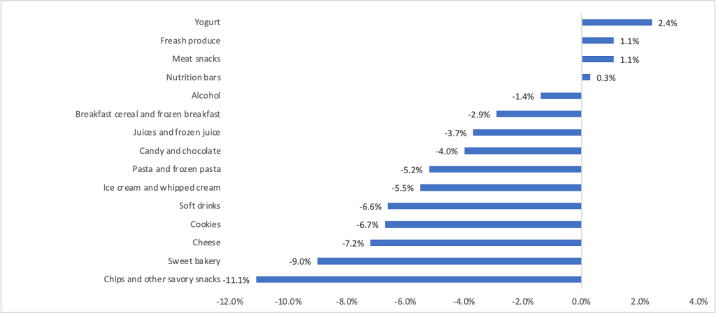
The study finds that households with at least one person using a GLP–1 drug reduced their total grocery shopping by 5.5 percent or $416. The study gathered data on changes in the categories of food that households were buying six months after at least one person in the household began using one of these drugs. The figure below is compiled from data in the study.
As expected, purchases of snacks declined. The category of “chips and other savor snacks” (bottom row in the figure) declined by more than 11 percent. Purchases of sweet bakery products, cheese, cookies, soft drinks, ice cream, and pasta all declined by more than 5 percent. Purchases of yogurt, fresh produce, meat snacks, and nutrition bars, all increased. An article in the Wall Street Journal noted that “food makers are starting to understand better and cater to, in some cases with products specifically designed for” users of this drug. The image below shows some of the new products that Nestle—a major candy producer—has introduced to appeal to users of GLP–1 drugs. Nestle’s Vital Pursuit line of frozen packaged foods contain high levels of protein and fiber.
It’s too early to gauge the full effects of GLP–1 drugs on consumer demand. But it’s already clear that GLP–1 drugs are a striking example of technological change affecting demand in a major industry
The pool at the All-Star Movie resort at Walt Disney World in Orlando, Florida (Photo from touringplans.com)
A recent article in the Wall Street Journal has the headline “Even Disney Is Worried About the High Cost of a Disney Vacation.” According to the article, “Some inside Disney worry that the company has become addicted to price hikes and has reached the limits of what middle-class Americans can afford ….”
As we discuss in Microeconomics, Chapter 15, the Walt Disney Company engages in price discrimination in a number of ways, by, for instance, charging more for ticket prices to its theme parks during the end-of-year holidays than on other days. Disney also offers hotels at different price levels, ranging from deluxe hotels like the Grand Floridian to more basic value hotels like the All-Star Movie Resort. In the case of hotels, some of the price difference is explained by differences in operating cost. Luxury hotels tend to have more amenities, including larger pools and restaurants on site, which raises their costs. Part of the difference in price, though, is the result of Disney estimating that people with higher incomes have a more inelastic demand for hotels than do people with lower incomes.
The Wall Street Journal article relies in part on data provided by Len Testa on his site touringplans.com. He notes that between 2018 and 2025, the percentage increase in the price Disney charged for staying at a value resort was less than the rate of inflation. In other words, the real price—the nominal price corrected for the effects of inflation—of staying at a Disney value resort decreased during that period. On the other hand, the percentage increase in the price Disney charged for staying at a deluxe was more than the rate of the inflation. So, the real price of staying at a Disney deluxe resort increased during this period.
One interpretation of these data is that over this period, Disney increased the extent of the price discrimination it was practicing with respect to hotel prices. It increased the gap between the price the families with more inelastic demand for Disney hotels pay and the price families with more elastic demand for Disney hotels pay. The article quotes Josh D’Amaro, who is the Disney executive in charge of the company’s theme parks, as saying “we intentionally offer a wide variety of ticket, hotel and dining options to welcome as many families as possible, whatever their budget.”
At the close of stock trading on Friday, January 24 at 4 pm EST, Nvidia’s stock had a price of $142.62 per share. When trading reopened at 9:30 am on Monday, January 27, Nvidia’s stock price plunged to $127.51. The total value of all Nvidia’s stock (the firm’s market capitalization or market cap) dropped by $589 billion—the largest one day drop in market cap in history. The following figure from the Wall Street Journal shows movements in Nvidia’s stock price over the past six months.
What happened to cause should a dramatic decline in Nvidia’s stock price? As we discuss in Macroeconomics, Chapter 6 (Economics, Chapter 8, and Money, Banking, and the Financial System, Chapter 6), Nividia’s price of $142.62 at the close of trading on January 24—like the price of any publicly traded stock—reflected all the information available to investors about the company. For the company’s stock to have declined so sharply at the beginning of the next trading day, important new information must have become available—which is exactly what happened.
As we discussed in this blog post from last October, Nvidia has been very successful in producing state-of-the-art computer chips that power the most advanced generative artificial intelligence (AI) software. Even after Monday’s plunge in the value of its stock, Nvidia still had a market cap of nearly $3.5 trillion at the end of the day. It wasn’t news that DeepSeek, a Chinese AI company had produced AI software called R1 that was similar to ChatGTP and other AI software produced by U.S. companies. The news was that R1—the latest version of the software is called V3—appeared to be comparable in many ways to the AI software produced by U.S. firms, but had been produced by DeepSeek despite not using the state-of-the-art Nvidia chips used in those AI programs.
The Biden administration had barred export to China of the newest Navidia chips to keep Chinese firms from surging ahead of U.S. firms in developing AI. DeepSeek claimed to have developed its software using less advanced chips and have trained its software at a much lower cost than U.S. firms have been incurring to train their software. (“Training” refers to the process by which engineers teach software to be able to accurately solve problems and answer questions.) Because DeepSeek’s costs are lower, the company charges less than U.S. AI firms do to use its computer infrastructure to handle business tasks like responding to consumer inquiries.
If the claims regarding DeepSeek’s software are accurate, then AI firms may no longer require the latest Nvidia chips and may be forced to reduce the prices they can charge firms for licensing their software. The demand for electricity generation may also decline if it turns out that the demand for AI data centers, which use very large amounts of power, will be lower than expected.
But on Monday it wasn’t yet clear whether the claims being made about DeepSeek’s software were accurate. Some industry observers speculated that, despite the U.S. prohibition on exporting the latest Nvidia chips to China, DeepSeek had managed to obtain them but was reluctant to admit that it had. There were also questions about whether DeepSeek had actually spent as little as it claimed in training its software.
What happens to the price of Nvidia’s stock during the rest of the week will indicate how investors are evaluating the claims DeepSeek made about its AI software.
Welcome to the first podcast for the Spring 2025 semester from the Hubbard/O’Brien Economics author team. Check back for Blog updates & future podcasts which will happen every few weeks throughout the semester.
Join authors Glenn Hubbard & Tony O’Brien as they offer thoughts on tariffs in advance of the beginning of the new administration. They discuss the positive and negative impacts of tariffs -and some of the intended consequences. They also look at the AI landscape and how its reshaping the US economy. Is AI responsible for recent increased productivity – or maybe just the impact of other factors. It should be looked at closely as AI becomes more ingrained in our economy.
The cover of Steven King’s novel The Stand. (Image from amazon.com)
In Microeconomics, Chapter 10, we have a section on “Pitfalls in Decision Making.” One of those pitfalls is the failure to ignore sunk costs. A sunk cost is one that has already been paid and cannot be recovered.
In his book On Writing: A Memoir of the Craft, King discusses his writing of The Stand (a book he describes as “the one my longtime readers still seem to like the best.”) At one point he had had trouble finishing the manuscript and was considering whether to stop working on the novel:
“If I’d had two or even three hundred pages of single-spaced manuscript instead of more than five hundred, I think I would have abandoned The Stand and gone on to something else—God knows I had done it before. But five hundred pages was too great an investment, both in time and in creative energy; I found it impossible to let go.”
King seems to have committed the error of ignoring sunk costs. The time and creative energy he had put into writing the 500 pages were sunk—whether he abandoned the manuscript or continued writing until the book was finished, he couldn’t get back the time and energy he had expanded on writing the first five hundred pages. That he had already written 300 pages or 500 pages wasn’t relevant to his decision because if a cost is sunk it doesn’t matter for decision making whether the cost is large or small.
Is it relevant in assessing King’s decision that in the end he did finish The Stand, the novel sold well—earning King substantial royalties—and his fans greatly admire the novel? Not directly because only with hindsight do we know that The Stand was successful. In deciding whether to finish the manuscript, King shouldn’t have worried about the cost of the time and energy he had already spent writing it. Instead, King should have compared the expected marginal cost of finishing the manuscript with the expected marginal benefit from completing the book. Note that the expected marginal benefit could include not only the royalty earnings from sales of the books, but also the additional appreciation he received from his fans for writing what turned out to be their favorite novel.
When King paused working on the manuscript after having written 500 pages, the marginal cost of finishing was the opportunity cost of not being able to spend those hours and creative energy writing a different book. Given the success of The Stand, the marginal benefit to King from completing the manuscript was almost certainly greater than the marginal cost. So, completing the manuscript was the correct decision, even if he made it for the wrong reason!