Acemoglu, Johnson, and Robinson Win the 2024 Nobel Prize in Economics

Daron Acemoglu and Simon Johnson (Credit: Acemoglu, Adam Glanzman; Johnson, courtesy of MIT, from news.mit.edu)

James Robinson (photo from news.uchicago.edu)

Many economic studies have a relatively limited objective. For instance, estimating the price elasticity of demand for soda in order to determine the incidence of a soda tax. Or estimating a Keynesian fiscal policy multiplier in order to determine the effects of a change in federal spending or taxes. (We consider the first topic in Microeconomics, Chapter 6, and the second topic in Macroeconomics, Chapter 16.)

Other economic studies consider much broader questions, such as why are some countries rich and other countries poor? As the late Nobel laureate Robert Lucas once wrote: “The consequences for human welfare involved in questions like these are simply staggering: Once one starts to think about them, it is hard to think about anything else.”

Today, the Royal Swedish Academy of Sciences awarded the 2024 Nobel Prize in Economic Sciences to Daron Acemoglu and Simon Johnson of MIT, and to James Robinson of the University of Chicago for “for studies of how institutions are formed and affect prosperity.” Acemoglu, Johnson, and Robinson (AJR) have published work highlighting the key importance of a country’s institutions in explaining whether the country has experienced sustained economic growth. Their work builds on earlier studies by the late Douglas North of Washington University in St. Louis, who received the Nobel Prize in 1993.

The institutional approach to economic growth differs from other approaches that focus on variables such as temperature, prevalence of disease, ethnic fragmentation, resource endowments, or governments adopting flawed development strategies in explaining differences in growth rates in per capita income across countries.

Two of AJR’s most discussed papers are “The Colonial Origins of Comparative Development: An Empirical Investigation,” which was published in the American Economic Review in 2001 (free download here), “Reversal of Fortune: Geography and Institutions in the Making of the Modern World Income Distribution,” which was published in the Quarterly Journal of Economics in 2002 (available here). In these papers, the authors argue that the institutions European countries established in their colonies helped determine economic growth in those countries even decades after colonization.

As with any analysis that covers many countries over long periods of time, AJR’s analysis of the effect of colonialism on economic growth has attracted critiques focused on whether the authors have gathered data properly and whether their data may be better explained with a different approach.

The authors, writing both separately and jointly, have explored many issues beyond the effects of colonialism on economic growth. The wide scope of their research can be seen by reviewing their curricula vitae, which can be found here, here, and here. The announcement by the Nobel committee can be found here.

(Probably) the Final Word on the Non-Recession of 2022

Image generated by GTP-4o to illustrate GDP.

About one month after a calendar quarter ends, the Bureau of Economic Analyis (BEA) releases its advanced estimate of real GDP. In July 2022, the BEA’s advance estimates indicated that real GDP had declined in both the first and second quarters. A common definition of a recession is two consecutive quarters of declining real GDP. Accordingly, in mid-2022 there were a number of articles in the media suggesting that the U.S. economy was in a recession.

But, as we discussed at the time in this blog post, most economists don’t follow the popular definition of a recession as being two consecutive quarters of declining real GDP. Instead, as we discuss in Macroeconomics, Chapter 10, Section 10.3 (Economics, Chapter 20, Section 20.3), economists typically follow the definition of a recession used by the National Bureau of Economic Research (NBER): “A recession is a significant decline in activity spread across the economy, lasting more than a few months, visible in industrial production, employment, real income, and wholesale-retail trade.” 

During the first half of 2022, the other data that the NBER tracks were all expanding rather than contracting. So, it seemed safe to conclude that despite the declines in real GDP in those quarters, the U.S. economy was not, in fact, in a recession.

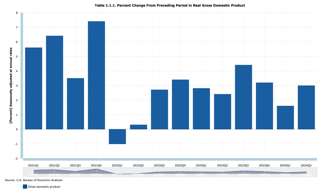
That conclusion was confirmed by the BEA in September 2024 when it released its most recent revisions of real GDP . As the following table shows, although the BEA still estimates that real GDP fell during the first quarter of 2022, it now estimates that it increased during the second quarter.

In the earlier post from 2022, we also noted that the BEA publishes data on gross domestic income (GDI), as well as on GDP. As we discuss in Chapter 8, Section 8.1, when considering the circular-flow diagram, the value of every final good and service produced in the economy (GDP) should equal the value of all the income in the economy resulting from that production (GDI). The BEA has designed the two measures to be identical by including in GDI some non-income items, such as sales taxes and depreciation. But as we discuss in the Apply the Concept, “Should We Pay More Attention to Gross Domestic Income?” GDP and GDI are compiled by the BEA from different data sources and can sometimes significantly diverge. 

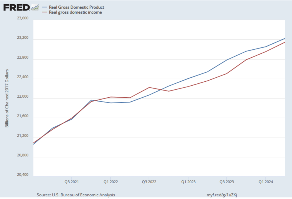
We noted that although, according to the BEA’s advance estimates, real GDP declined during the first two quarters of 2022, real GDI increased. The following figure shows movements in real GDP and real GDI using the current estimates from the BEA. The revised estimates now show real GDP falling the first quarter of 2021 and increasing in the second quarter while real GDI is still estimated as rising in both quarters. The revisions closed some of the gap between real GDP and real GDI during this period by increasing the estimate for real GDP, which indicates that the advance estimate of real GDI was giving a more accurate measure of what was happening in the U.S. economy.

The figure shows that the revised estimates indicate that real GDP and real GDI moved closely together during 2021, differed somewhat during 2022—with real GDI being greater than real GDP—and differed more substantially during 2023 and 2024—with real GDP now being greater than real GDI. Because the two measures should be the same, we can expect that further revisions by the BEA will bring the two measures closer together.

It’s even possible, but unlikely, that further revisions of the data for 2022 could again present us with the paradox of real GDP declining for two quarters despite other measures of economic activity expanding.

9/15/24 Podcast – Authors Glenn Hubbard & Tony O’Brien provide a Macroeconomics update & highlight next steps in advance of FOMC meeting.

Welcome to the first podcast for the Fall 2024 semester from the Hubbard/O’Brien Economics author team. Check back for Blog updates & future podcasts which will happen every few weeks throughout the semester.

Join authors Glenn Hubbard & Tony O’Brien as they provide an update on the Macroeconomy. They offer thoughts on the likelihood of a soft landing and whether the actions of the Federal Reserve helped or hindered that process. The monetary and fiscal challenges facing the new administration are real and the Fed will begin its process of rate-cutting this week in the upcoming FOMC meeting. Gain insight into this evolving situation by listening to this podcast. Click HERE to access the podcast.

https://on.soundcloud.com/ywr6WfPPKPofeHr19

Latest Jobs Report May Indicate the Labor Market Is Weakening

Image generated by ChatGTP 4o.

Recent macroeconomic data have been sending mixed signals about the state of the U.S. economy. The growth in real GDP, industrial production, retail sales, and real consumption spending has been slowing. Growth in employment has been a bright spot—showing steady net increases in job growth above the level necessary to keep up with population growth. Even here, though, as we discuss in a recent blog post, the data may be overstating the actual strength of the labor market.

This morning (July 5), the Bureau of Labor Statistics (BLS) released its “Employment Situation” report (often referred to as the “jobs report”) for June, which, while seemingly indicating continued strong job growth, also provides some indications that the labor market may be weakening. The jobs report has two estimates of the change in employment during the month: one estimate from the establishment survey, often referred to as the payroll survey, and one from the household survey. As we discuss in Macroeconomics, Chapter 9, Section 9.1 (Economics, Chapter 19, Section 19.1), many economists and policymakers at the Federal Reserve believe that employment data from the establishment survey provides a more accurate indicator of the state of the labor market than do either the employment data or the unemployment data from the household survey. (The groups included in the employment estimates from the two surveys are somewhat different, as we discuss in this post.)

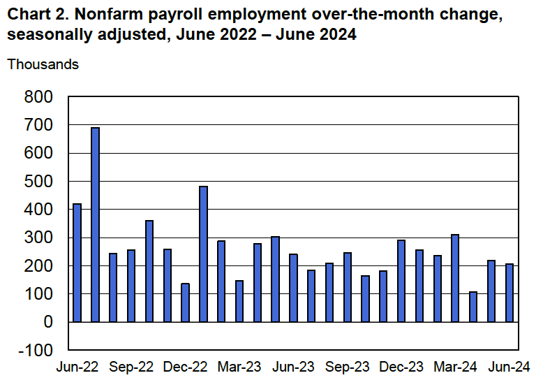
According to the establishment survey, there was a net increase of 206,000 jobs during April. This increase was a little above the increase of 1900,000 to 200,000 that economists had forecast in surveys by the Wall Street Journal and bloomberg.com. The following figure, taken from the BLS report, shows the monthly net changes in employment for each month during the past to years.

It’s notable that the previously reported increases in employment for April and May were revised downward by 110,000 jobs, or by about 25 percent. (The BLS notes that: “Monthly revisions result from additional reports received from businesses and government agencies since the last published estimates and from the recalculation of seasonal factors.”) As we’ve discussed in previous posts (most recently here), revisions to the payroll employment estimates can be particularly large at the beginning of a recession.

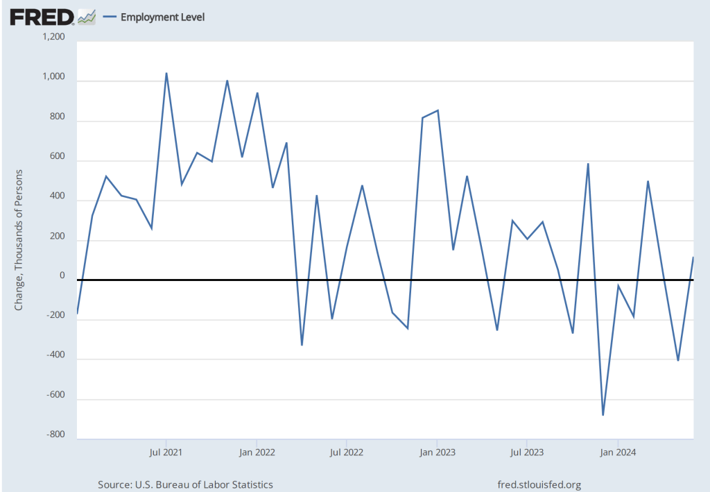
As the following figure shows, the net change in jobs from the household survey moves much more erratically than does the net change in jobs in the establishment survey. The net increase in jobs as measured by the household survey increased from –408,000 in May (that is, employment by this measure fell during May) to 116,000 in June.

Note that the BLS also reports a survey for household employment adjusted to conform to the concepts and definitions used to construct the payroll employment series. After this adjustment, over the past 12 months household employment has increased by 32.5 million less than has payroll employment. Clearly, this is a very large discrepancy and may be indicating that the payroll survey is substantially overstating growth in employment.

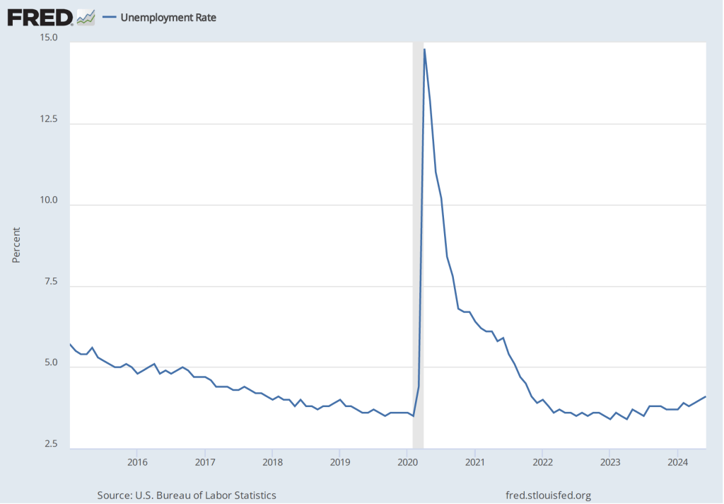
The unemployment rate, which is also reported in the household survey, ticked up slightly from 4.0 percent to 4.1 percent. Although still low by historical standards, June was the fourth consecutive month in which the unemployment rate increased.

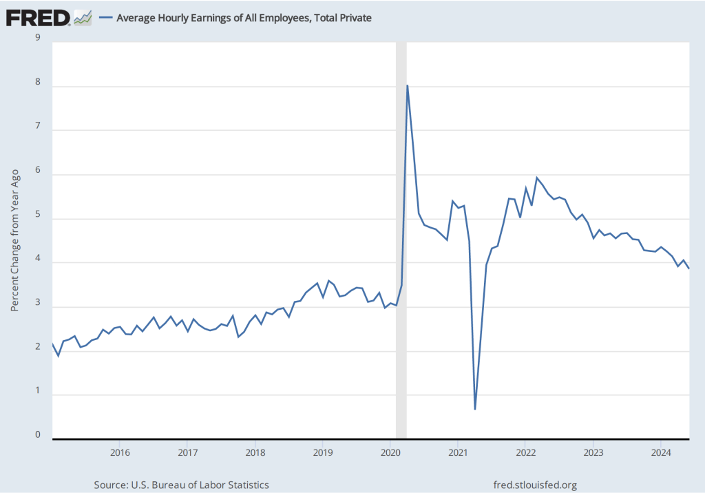
The establishment survey also includes data on average hourly earnings (AHE). As we note in this post, many economists and policymakers believe the employment cost index (ECI) is a better measure of wage pressures in the economy than is the AHE. The AHE does have the important advantage that it is available monthly, whereas the ECI is only available quarterly. The following figure show the percentage change in the AHE from the same month in the previous year. The 3.9 percent increase for June continues a downward trend that began in January and is the smallest increase since June 2021.

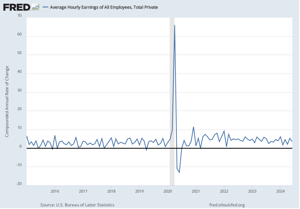
The following figure shows wage inflation calculated by compounding the current month’s rate over an entire year. (The figure above shows what is sometimes called 12-month wage inflation, whereas this figure shows 1-month wage inflation.) One-month wage inflation is much more volatile than 12-month inflation—note the very large swings in 1-month wage inflation in April and May 2020 during the business closures caused by the Covid pandemic.

The 1-month rate of wage inflation of 3.5 percent in June is a significant decrease from the 5.3 percent rate in May, although it’s unclear whether the decline was an additional sign that the labor market is weakening or reflected the greater volatility in wage inflation when calculated this way.

What effect is today’s job reports likely to have on the Fed’s policy-making Federal Open Market Committee as it considers changes in its target for the federal funds rate? As always, it’s a good idea not to rely too heavily on a single data point—particularly because, as we noted earlier, the establishment survey employment data is subject to substantial revisions. But the Wall Street Journal’s headline that the “Case for September Rate Cut Builds After Slower Jobs Data,” seems likely to be accurate.

4/5/24 Podcast – Authors Glenn Hubbard & Tony O’Brien react to the newest Friday Jobs Report for March & discuss next steps for the Economy.

Join authors Glenn Hubbard & Tony O’Brien as they react to the jobs report of over 300K jobs created which was way over expectations of about 200K. They consider the impact of this report as the Fed considers the next steps for the economy. Are we on a glide path for a soft landing at 2% inflation or will the Fed reconsider its long-standing target by adopting a higher 3% target? Glenn and Tony offer interesting viewpoints on where this is headed.

Key Macro Data Series during the Time Since the Arrival of Covid–19 in the United States

A bookstore in New York City closed during Covid. (Photo from the New York Times)

Four years ago, in mid-March 2020, Covid–19 began to significantly affect the U.S. economy, with hospitalizations rising and many state and local governments closing schools and some businesses. In this blog post we review what’s happened to key macro variables during the past four years. Each monthly series starts in February 2020 and the quarterly series start in the fourth quarter of 2019.

Production

Real GDP declined by 5.8 percent from the fourth quarter of 2019 to the first quarter of 2020 and by an additional 28.0 percent from the first quarter of 2020 to the second quarter. This decline was by far the largest in such a short period in the history of the United States. From the second quarter to the third quarter of 2020, as businesses began to reopen, real GDP increased by 34.8 percent, which was by far the largest increase in a single quarter in U.S. history.

Industrial production followed a similar—although less dramatic—path to real GDP, declining by 16.8 percent from February 2020 to April 2020 before increasing by 12.3 percent from April 2020 to June 2020. Industrial production did not regain its February 2020 level until March 2022. The swings in industrial production were smaller than the swings in GDP because industrial production doesn’t include the output of the service sector, which includes firms like restaurants, movie theaters, and gyms that were largely shutdown in some areas. (Industrial production measures the real output of the U.S. manufacturing, mining, and electric and gas utilities industries. The data are issued by the Federal Reserve and discussed here.)

Employment

Nonfarm payroll employment, collected by the Bureau of Labor Statistics (BLS) in its establishment survey, followed a path very similar to the path of production. Between February and April 2020, employment declined by an astouding 22 million workers, or by 14.4 percent. This decline was by far the largest in U.S. history over such a short period. Employment increased rapidly beginning in April but didn’t regain its February 2020 level until June 2022.

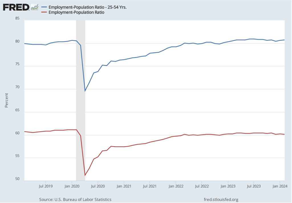
The employment-population ratio measures the percentage of the working-age population that is employed. It provides a more comprehensive measure of an economy’s utilization of available labor than does the total number of people employed. In the following figure, the blue line shows the employment-population ratio for the whole working-age population and the red line shows the employment-population ratio for “prime age workers,” those aged 25 to 54.

For both groups, the employment-population ratio plunged as a result of Covid and then slowly recovered as the production began increasing after April 2020. The employment-population ratio for prime age workers didn’t regain its February 2020 value until February 2023, an indication of how long it took the labor market to fully overcome the effects of the pandemic. As of February 2024, the employment-population ratio for all people of working age hasn’t returned to its February 2020 value, largely because of the aging of the U.S. population.

Average weekly hours worked followed an unusual pattern, declining during March 2020 but then increasing to beyond its February 2020 level to a peak in April 2021. This increase reflects firms attempting to deal with a shortage of workers by increasing the hours of those people they were able to hire. By April 2023, average weekly hours worked had returned to its February 2020 level.

Income

Real average hourly earnings surged by more than six percent between February and April 2020—a very large increase over a two-month period. But some of the increase represented a composition effect—as workers with lower incomes in services industries such as restaurants were more likely to be out of work during this period—rather than an actual increase in the real wages received by people employed during both months. (Real average hourly earnings are calculated by dividing nominal average hourly earnings by the consumer price index (CPI) and multiplying by 100.)

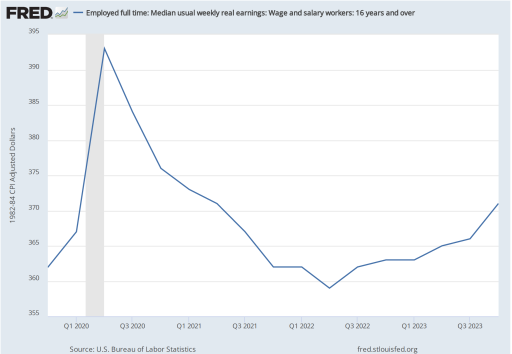
Median weekly real earnings, because it is calculated as a median rather than as an average (or mean), is less subject to composition effects than is real average hourly earnings. Median weekly real earnings increased sharply between February and April of 2020 before declining through June 2022. Earnings then gradually increased. In February 2024 they were 2.5 percent higher than in February 2020.

Inflation

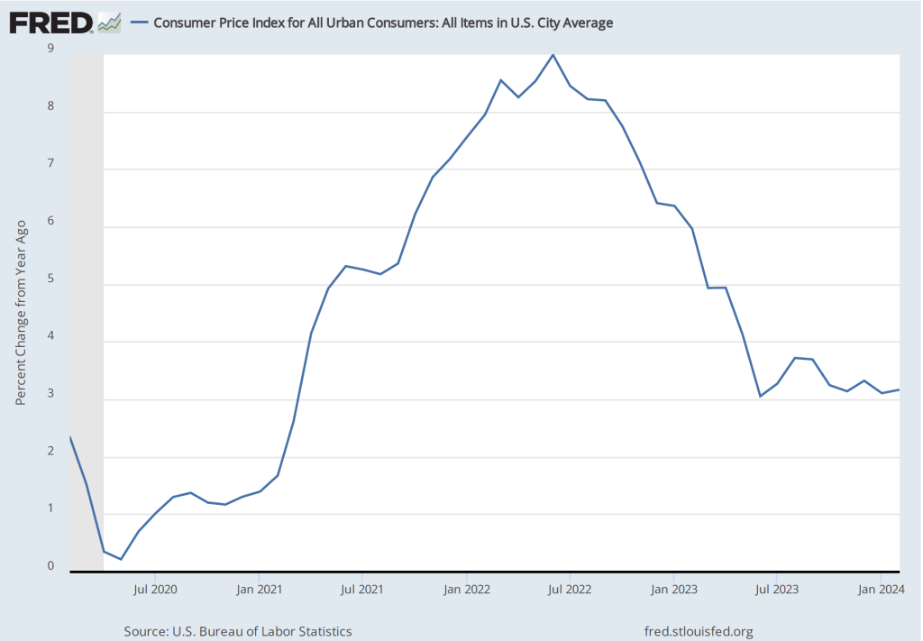
The inflation rate most commonly mentioned in media reports is the percentage change in the CPI from the same month in the previous year. The following figure shows that inflation declined from February to May 2020. Inflation then began to rise slowly before rising rapidly beginning in the spring of 2021, reaching a peak in June 2022 at 9.0 percent. That inflation rate was the highest since November 1981. Inflation then declined steadily through June 2023. Since that time it has fluctuated while remaining above 3 percent.

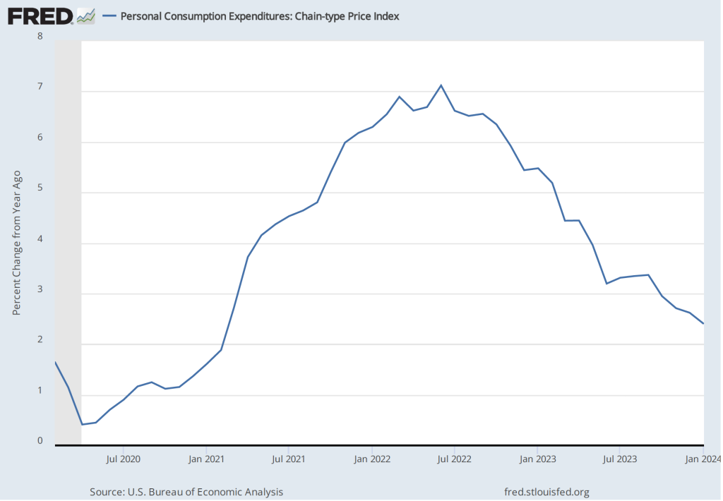
As we discuss in Macroeconomics, Chapter 15, Section 15.5 (Economics, Chapter 25, Section 25.5), the Federal Reserve gauges its success in meeting its goal of an inflation rate of 2 percent using the personal consumption expenditures (PCE) price index. The following figure shows that PCE inflation followed roughly the same path as CPI inflation, although it reached a lower peak and had declined below 3 percent by November 2023. (A more detailed discussion of recent inflation data can be found in this post and in this post.)

Monetary Policy

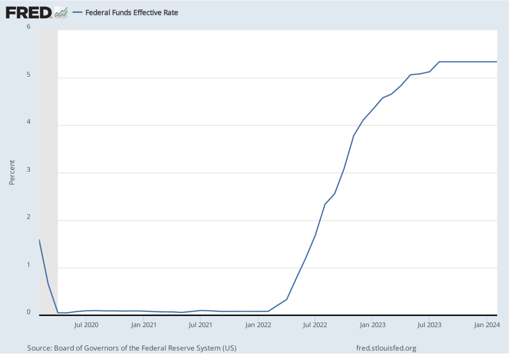
The following figure shows the effective federal funds rate, which is the rate—nearly always within the upper and lower bounds of the Fed’s target range—that prevails during a particular period in the federal funds market. In March 2020, the Fed cut its target range to 0 to 0.25 percent in response to the economic disruptions caused by the pandemic. It kept the target unchanged until March 2022 despite the sharp increase in inflation that had begun a year earlier. The members of the Federal Reserve’s Federal Open Market Committee (FOMC) had initially hoped that the surge in inflation was largely caused by disuptions to supply chains and would be transitory, falling as supply chains returned to normal. Beginning in March 2022, the FOMC rapidly increased its target range in response to continuing high rates of inflation. The targer range reached 5.25 to 5.50 percent in July 2023 where it has remained through March 2024.


Although the money supply is no longer the focus of monetary policy, some economists have noted that the rate of growth in the M2 measure of the money supply increased very rapidly just before the inflation rate began to accelerate in the spring of 2021 and then declined—eventually becoming negative—during the period in which the inflation rate declined.

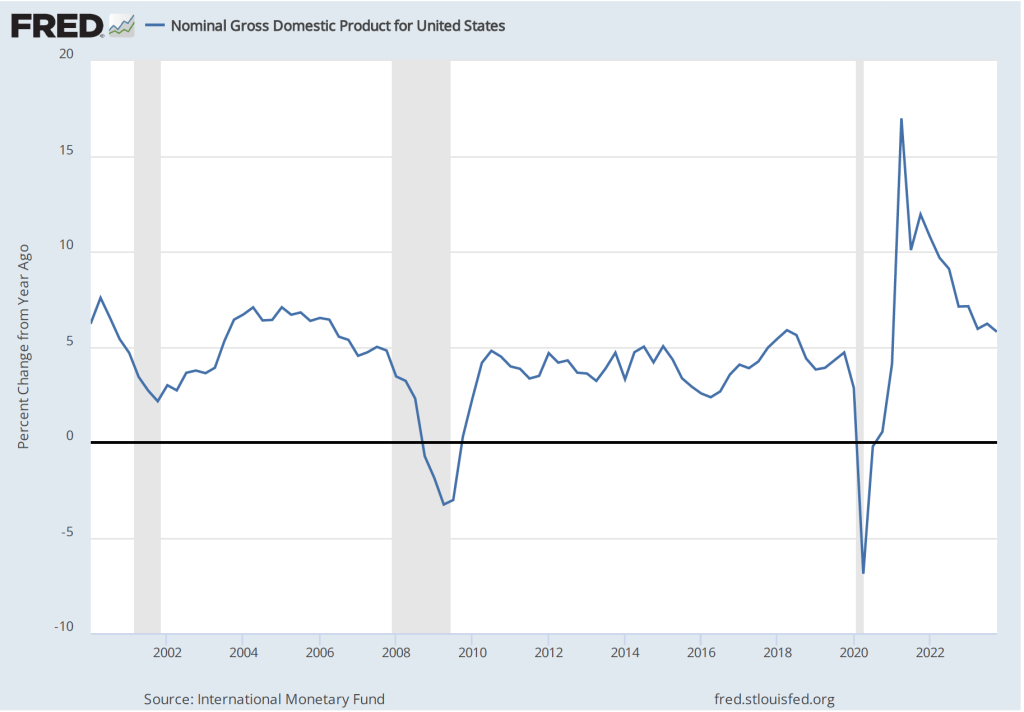
As we discuss in the new 9th edition of Macroeconomics, Chapter 15, Section 15.5 (Economics, Chapter 25, Section 25.5), some economists believe that the FOMC should engage in nominal GDP targeting. They argue that this approach has the best chance of stabilizing the growth rate of real GDP while keeping the inflation rate close to the Fed’s 2 percent target. The following figure shows the economy experienced very high rates of inflation during the period when nominal GDP was increasing at an annual rate of greater than 10 percent and that inflation declined as the rate of nominal GDP growth declined toward 5 percent, which is closer to the growth rates seen during the 2000s. (This figure begins in the first quarter of 2000 to put the high growth rates in nominal GDP of 2021 and 2022 in context.)

Fiscal Policy

As we discuss in the new 9th edition of Macroeconomics, Chapter 15 (Economics, Chapter 25), in response to the Covid pandemic Congress and Presidents Trump and Biden implemented the largest discretionary fiscal policy actions in U.S. history. The resulting increases in spending are reflected in the two spikes in federal government expenditures shown in the following figure.

The initial fiscal policy actions resulted in an extraordinary increase in federal expenditures of $3.69 trillion, or 81.3 percent, from the first quarter to the second quarter of 2020. This was followed by an increase in federal expenditures of $2.31 trillion, or 39.4 percent, from the fourth quarter of 2020 to the first quarter of 2021. As we recount in the text, there was a lively debate among economists about whether these increases in spending were necessary to offest the negative economic effects of the pandemic or whether they were greater than what was needed and contributed substantially to the sharp increase in inflation that began in the spring of 2021.

Saving

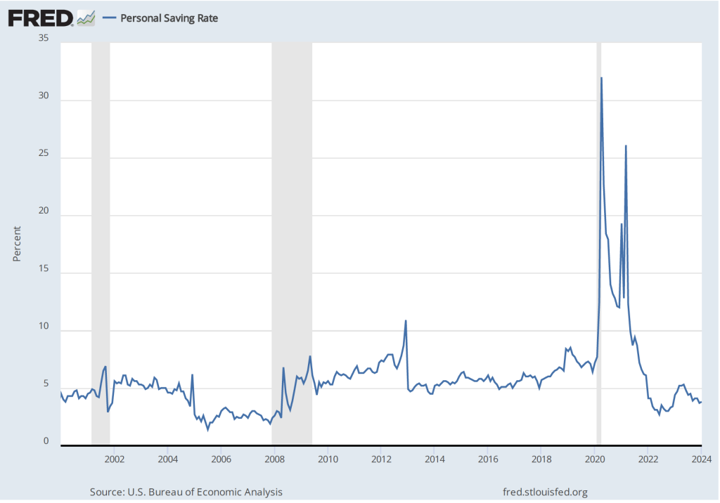
As a result of the fiscal policy actions of 2020 and 2021, many households received checks from the federal government. In total, the federal government distributed about $80o billion directly to households. As the figure shows, one result was to markedly increase the personal saving rate—measured as personal saving as a percentage of disposable personal income—from 6.4 percent in December 2019 to 22.0 in April 2020. (The figure begins in January 2020 to put the size of the spike in the saving rate in perspective.) 

The rise in the saving rate helped households maintain high levels of consumption spending, particularly on consumer durables such as automobiles. The first of the following figure shows real personal consumption expenditures and the second figure shows real personal consumption expenditures on durable goods.

Taken together, these data provide an overview of the momentous macroeconomic events of the past four years.

Will the United States Experience a Sustained Boom in the Growth Rate of Labor Productivity?

Blue Planet Studio/Shutterstock

Recent articles in the business press have discussed the possibility that the U.S. economy is entering a period of higher growth in labor productivity:

“Fed’s Goolsbee Says Strong Hiring Hints at Productivity Growth Burst” (link)

“US Productivity Is on the Upswing Again. Will AI Supercharge It?” (link)

“Can America Turn a Productivity Boomlet Into a Boom?” (link)

In Macroeconomics, Chapter 16, Section 16.7 (Economics, Chapter 26, Section 26.7), we highlighted  the role of growth in labor productivity in explaining the growth rate of real GDP using the following equations. First, an identity:

Real GDP = Number of hours worked x (Real GDP/Number of hours worked),

where (Real GDP/Number of hours worked) is labor productivity.

And because an equation in which variables are multiplied together is equal to an equation in which the growth rates of these variables are added together, we have:

Growth rate of real GDP = Growth rate of hours worked + Growth rate of labor productivity

From 1950 to 2023, real GDP grew at annual average rate of 3.1 percent. In recent years, real GDP has been growing more slowly. For example, it grew at a rate of only 2.0 percent from 2000 to 2023. In February 2024, the Congressional Budget Office (CBO) forecasts that real GDP would grow at 2.0 percent from 2024 to 2034. Although the difference between a growth rate of 3.1 percent and a growth rate of 2.0 percent may seem small, if real GDP were to return to growing at 3.1 percent per year, it would be $3.3 trillion larger in 2034 than if it grows at 2.0 percent per year. The additional $3.3 trillion in real GDP would result in higher incomes for U.S. residents and would make it easier for the federal government to reduce the size of the federal budget deficit and to better fund programs such as Social Security and Medicare. (We discuss the issues concerning the federal government’s budget deficit in this earlier blog post.)

Why has growth in real GDP slowed from a 3.1 percent rate to a 2.0 percent rate? The two expressions on the right-hand side of the equation for growth in real GDP—the growth in hours worked and the growth in labor productivity—have both slowed. Slowing population growth and a decline in the average number of hours worked per worker have resulted in the growth rate of hours worked to slow substantially from a rate of 2.0 percent per year from 1950 to 2023 to a forecast rate of only 0.4 percent per year from 2024 to 2034.

Falling birthrates explains most of the decline in population growth. Although lower birthrates have been partially offset by higher levels of immigration in recent years, it seems unlikely that birthrates will increase much even in the long run and levels of immigration also seem unlikely to increase substantially in the future. Therefore, for the growth rate of real GDP to increase significantly requires increases in the rate of growth of labor productivity.
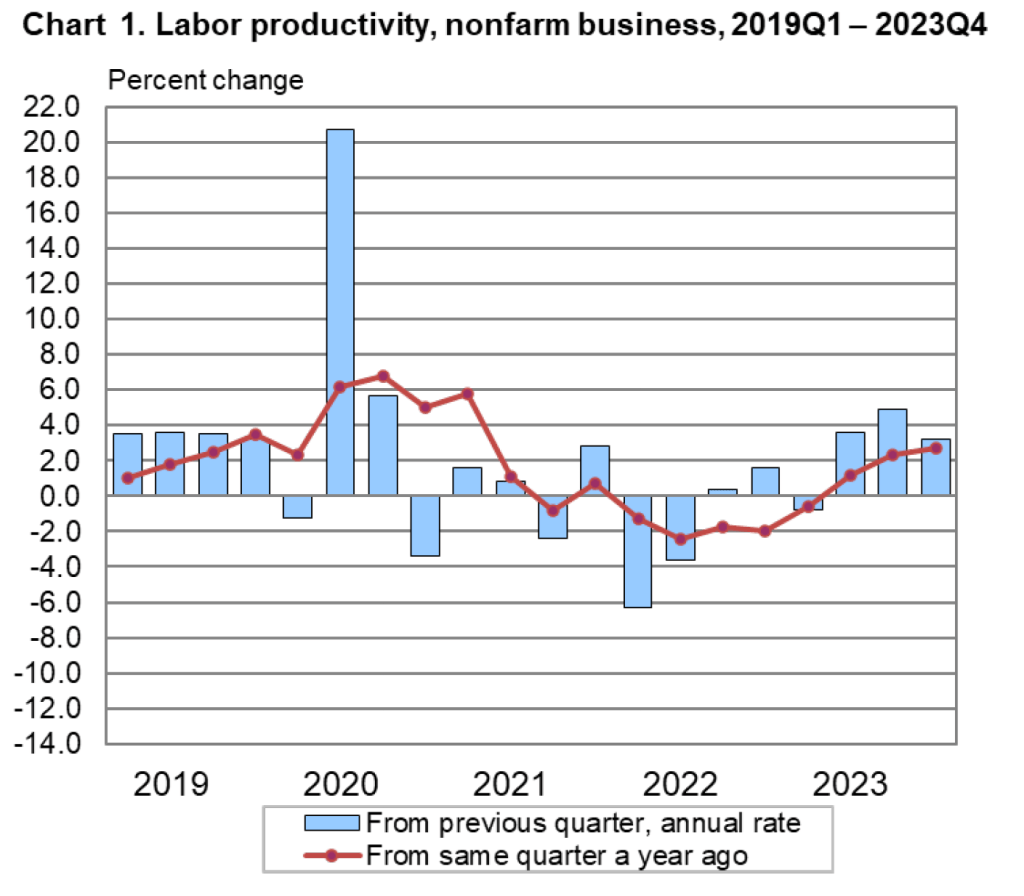
The Bureau of Labor Statistics (BLS) publishes quarterly data on labor productivity. (Note that the BLS series is for labor productivity in the nonfarm business sector rather than for the whole economy. Output of the nonfarm business sector excludes output by government, nonprofit businesses, and households. Over long periods, growth in real GDP per hour worked and growth in real output of the nonfarm business sector per hour worked have similar trends.) The following figure is taken from the BLS report “Productivty and Costs,” which was released on February 1, 2024.

Note that the growth in labor productivity increased during the last three quarters of 2023, whether we measure the growth rate as the percentage change from the same quarter in the previous year or as growth in a particular quarter expressed as anual rate. It’s this increase in labor productivity during 2023 that has led to speculation that labor productivity might be entering a period of higher growth. The following figure shows labor productivity growth, measured as the percentage change from the same quarter in the previous year for the whole period from 1950 to 2023.

The figure indicates that labor productivity has fluctuated substantially over this period. We can note, in particular, productivity growth during two periods: First, from 2011 to 2018, labor productivity grew at the very slow rate of 0.9 percent per year. Some of this slowdown reflected the slow recovery of the U.S. economy from the Great Recession of 2007-2009, but the slowdown persisted long enough to cause concern that the U.S. economy might be entering a period of stagnation or very slow growth.
Second, from 2019 through 2023, labor productivity went through very large swings. Labor productivity experienced strong growth during 2019, then, as the Covid-19 pandemic began affecting the U.S. economy, labor productivity soared through the first half of 2021 before declining for five consecutive quarters from the first quarter of 2022 through the first quarter of 2023—the first time productivity had fallen for that long a period since the BLS first began collecting the data. Although these swings were particularly large, the figure shows that during and in the immediate aftermath of recessions labor productivity typically fluctuates dramatically. The reason for the fluctuations is that firms can be slow to lay workers off at the beginning of a recession—which causes labor productivity to fall—and slow to hire workers back during the beginning of an economy recovery—which causes labor productivity to rise. 

Does the recent increase in labor productivity growth represent a trend? Labor productivity, measured as the percentage change since the same quarter in the previous year, was 2.7 percent during the fourth quarter of 2023—higher than in any quarter since the first quarter of 2021. Measured as the percentage change from the previous quarter at an annual rate, labor productivity grew at a very high average rate of 3.9 during the last three quarters of 2023. It’s this high rate that some observers are pointing to when they wonder whether growth in labor productivity is on an upward trend.

As with any other economic data, you should use caution in interpreting changes in labor productivity over a short period. The productivity data may be subject to large revisions as the two underlying series—real output and hours worked—are revised in coming months. In addition, it’s not clear why the growth rate of labor productivity would be increasing in the long run. The most common reasons advanced are: 1) the productivity gains from the increase in the number of people working from home since the pandemic, 2) businesses’ increased use of artificial intelligence (AI), and 3) potential efficiencies that businesses discovered as they were forced to operate with a shortage of workers during and after the pandemic.

To this point it’s difficult to evaluate the long-run effects of any of these factors. Wconomists and business managers haven’t yet reached a consensus on whether working from home increases or decreases productivity. (The debate is summarized in this National Bureau of Economic Research Working Paper, written by Jose Maria Barrero of Instituto Tecnologico Autonomo de Mexico, and Steven Davis and Nicholas Bloom of Stanford. You may need to access the paper through your university library.)

Many economists believe that AI is a general purpose technology (GPT), which means that it may have broad effects throughout the economy. But to this point, AI hasn’t been adopted widely enough to be a plausible cause of an increase in labor productivity. In addition, as Erik Brynjolfsson and Daniel Rock of MIT and Chad Syverson of the University of Chicago argue in this paper, the introduction of a GPT may initially cause productivity to fall as firms attempt to use an unfamiliar technology. The third reason—efficiency gains resulting from the pandemic—is to this point mainly anecdotal. There are many cases of businesses that discovered efficiencies during and immediately after Covid as they struggled to operate with a smaller workforce, but we don’t yet know whether these cases are sufficiently common to have had a noticeable effect on labor productivity.

So, we’re left with the conclusion that if the high labor productivity growth rates of 2023 can be maintained, the growth rate of real GDP will correspondingly increase more than most economists are expecting. But it’s too early to know whether recent high rates of labor productivty growth are sustainable.

Glenn’s Presentation at the ASSA Session on “The U.S. Economy: Growth, Stagnation or Financial Crisis and Recession?”

Glenn participated in this session hosted by the Society of Policy Modeling and the American Economic Association of Economic Educators and moderated by Dominick Salvatore of Fordham University. (Link to the page for this session in the ASSA program.)

Also making presentations at the session were Robert Barro of Harvard University, Janice Eberly of Northwestern University, Kenneth Rogoff of Harvard University, and John Taylor of Stanford University.

Here is the abstract for Glenn’s presentation:

Economic growth is foundational for living standards and as an objective for economic policy. The emergence of Artificial Intelligence as a General Purpose Technology, on the one hand, and a number of demographic and budget challenges, on the other hand, generate an unusually wide range of future economic outcomes. I focus on key ‘policy’ and ‘political economy’ considerations that increase the likelihood of a more favorable growth path given pre-existing trends and technological possibilities. By ‘policy,’ I consider mechanisms enabling growth through research, taxation, the scope of regulation, and competition. By ‘political economy’ factors, I consider mechanisms to increase economic participation in support of growth and policies that enhance it. I argue that both sets of mechanisms are necessary for a viable pro-growth economic policy framework.

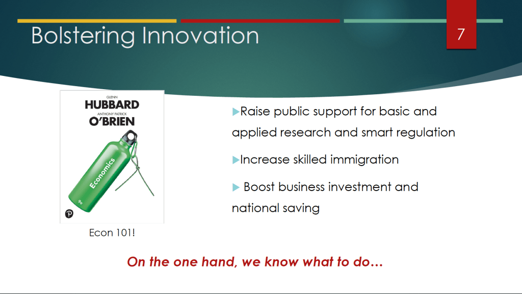
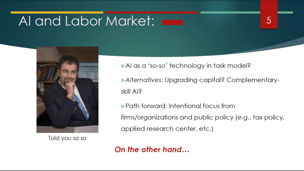
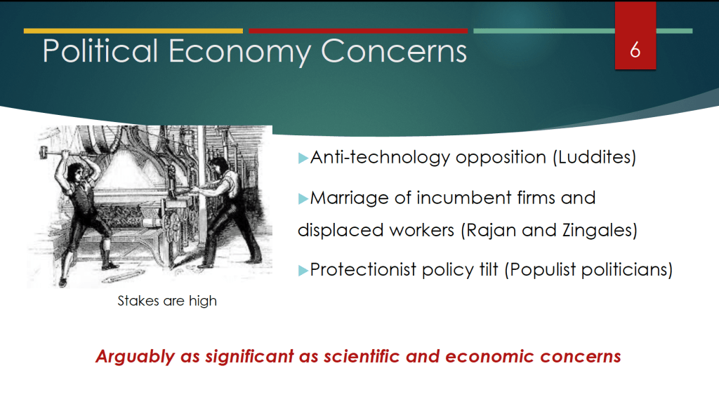
These slides from the presentation highlight some of Glenn’s key points. (Note the cover of the new 9th edition of the textbook in slide 7!)

The Roman Emperor Vespasian Fell Prey to the Lump-of-Labor Fallacy

Bust of the Roman Emperor Vespasian. (Photo from en.wikipedia.org.)

Some people worry that advances in artificial intelligence (AI), particularly the development of chatbots will permanently reduce the number of jobs available in the United States. Technological change is often disruptive, eliminating jobs and sometimes whole industries, but it also creates new industries and new jobs. For example, the development of mass-produced, low-priced automobiles in the early 1900s wiped out many jobs dependent on horse-drawn transportation, including wagon building and blacksmithing. But automobiles created many new jobs not only on automobile assembly lines, but in related industries, including repair shops and gas stations.

Over the long run, total employment in the United States has increased steadily with population growth, indicating that technological change doesn’t decrease the total amount of jobs available. As we discuss in Microeconomics, Chapter 16 (also Economics, Chapter 16), fears that firms will permanently reduce their demand for labor as they increase their use of the capital that embodies technological breakthroughs, date back at least to the late 1700s in England, when textile workers known as Luddites—after their leader Ned Ludd—smashed machinery in an attempt to save their jobs. Since that time, the term Luddite has described people who oppose firms increasing their use of machinery and other capital because they fear the increases will result in permanent job losses.

Economists believe that these fears often stem from the lump-of-labor fallacy, which holds that there is only a fixed amount of work to be performed in the economy. So the more work that machines perform, the less work that will be available for people to perform. As we’ve noted, though, machines are substitutes for labor in some uses—such as when chatbot software replace employees who currently write technical manuals or computer code—they are also complements to labor in other jobs—such as advising firms on how best to use chatbots. 

The lump-of-labor fallacy has a long history, probably because it seems like common sense to many people who see the existing jobs that a new technology destroys, without always being aware of the new jobs that the technology creates. There are historical examples of the lump-of-labor fallacy that predate even the original Luddites.

For instance, in his new book Pax: War and Peace in Rome’s Golden Age, the British historian Tom Holland (not to be confused with the actor of the same name, best known for portraying Spider-Man!), discusses an account by the ancient historian Suetonius of an event during the reign of Vespasian who was Roman emperor from 79 A.D. to 89 A.D. (p. 201):

“An engineer, so it was claimed, had invented a device that would enable columns to be transported to the summit of the [Roman] Capitol at minimal cost; but Vespasian, although intrigued by the invention, refused to employ it. His explanation was a telling one. ‘I have a duty to keep the masses fed.’”

Vespasian had fallen prey to the lump-of-labor fallacy by assuming that eliminating some of the jobs hauling construction materials would reduce the total number of jobs available in Rome. As a result, it would be harder for Roman workers to earn the income required to feed themselves.

Note that, as we discuss in Macroeconomics, Chapters 10 and 11 (also Economics, Chapter 20 and 21), over the long-run, in any economy technological change is the main source of rising incomes. Technological change increases the productivity of workers and the only way for the average worker to consume more output is for the average worker to produce more output. In other words, most economists agree that the main reason that the wages—and, therefore, the standard of living—of the average worker today are much higher than they were in the past is that workers today are much more productive because they have more and better capital to work with.
Although the Roman Empire controlled most of Southern and Western Europe, the Near East, and North Africa for more than 400 years, the living standard of the average citizen of the Empire was no higher at the end of the Empire than it had been at the beginning. Efforts by emperors such as Vespasian to stifle technological progress may be part of the reason why. 
10/21/23 Podcast – Authors Glenn Hubbard & Tony O’Brien reflect on the Fed’s efforts to execute the soft-landing.

Join authors Glenn Hubbard & Tony O’Brien as they reflect on the Fed’s efforts to execute the soft landing, ponder if the effect will stick, and wonder if future economies will be tethered to an anchor point above two percent.