

Happy New Year from Hubbard and O’Brien Economics!


Image created by ChatGTP
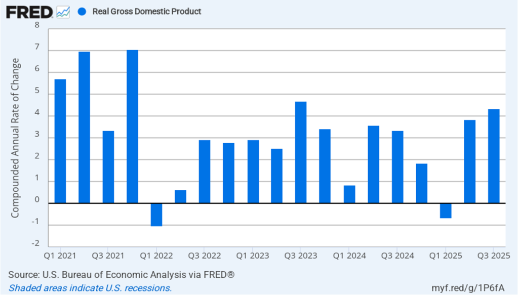
This morning (December 23), the Bureau of Economic Analysis (BEA) released its initial estimate of real GDP for the third quarter of 2025. (The report can be found here.) The BEA estimates that real GDP increased in the third quarter by 4.3 percent measured at an annual rate. Economists surveyed by FactSet had forecast a 3.2 percent increase. Real GDP experienced strong growth for the second quarter in a row, following an estimated 0.6 percent decline in the first quarter of 2025. The following figure shows the estimated rates of GDP growth in each quarter beginning with the first quarter of 2021.
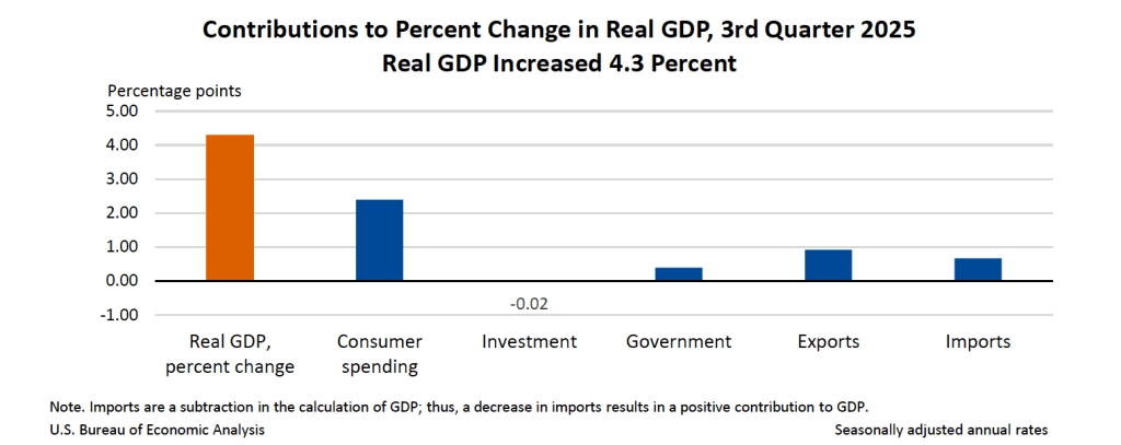
As the following figure—taken from the BEA report—shows, the growth in consumer spending in the third quarter was the most important factor contributing to the increase in real GDP. Increases in net exports and in government spending also contributed to GDP growth, while investment spending declined.
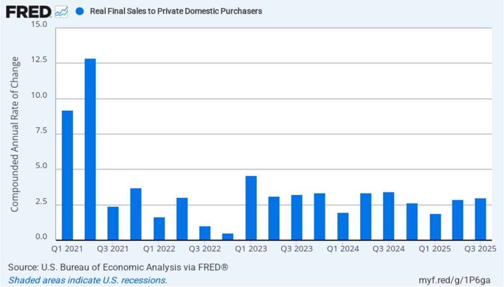
To better gauge the state of the economy, policymakers often prefer to strip out the effects of imports, inventory investment, and government purchases—which can be volatile—by looking at real final sales to private domestic purchasers, which includes only spending by U.S. households and firms on domestic production. As the following figure shows, real final sales to domestic purchasers increased by 3.0 percent at an annual rate in the third quarter, which was below the 4.3 percent increase in real GDP but still well above the U.S. economy’s expected long-run annual growth rate of 1.8 percent. Note also that real final sales to private domestic purchasers grew by 1.9 percent in the first quarter, during which real GDP declined. So this measure of output indicates solid growth during the first three quarters of the year.
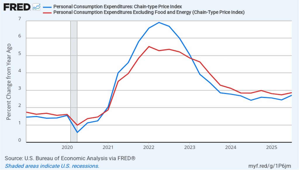
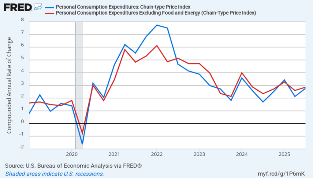
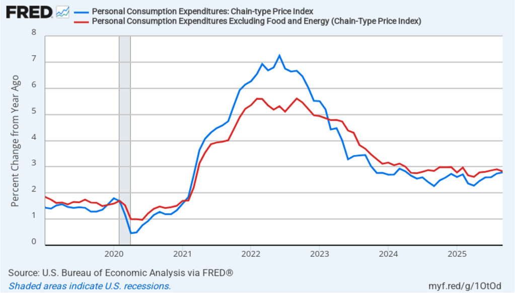
The BEA report this morning included quarterly data on the personal consumption expenditures (PCE) price index. The Fed relies on annual changes in the PCE price index to evaluate whether it’s meeting its 2 percent annual inflation target. The following figure shows headline PCE inflation (the blue line) and core PCE inflation (the red line)—which excludes energy and food prices—for the period since the first quarter of 2019, with inflation measured as the percentage change in the PCE from the same quarter in the previous year. In the third quarter, headline PCE inflation was 2.7 percent, up from 2.4 percent in the second quarter. Core PCE inflation in the third quarter was 2.9 percent, up from 2.7 percent in the second quarter. Both headline PCE inflation and core PCE inflation remained well above the Fed’s 2 percent annual inflation target.
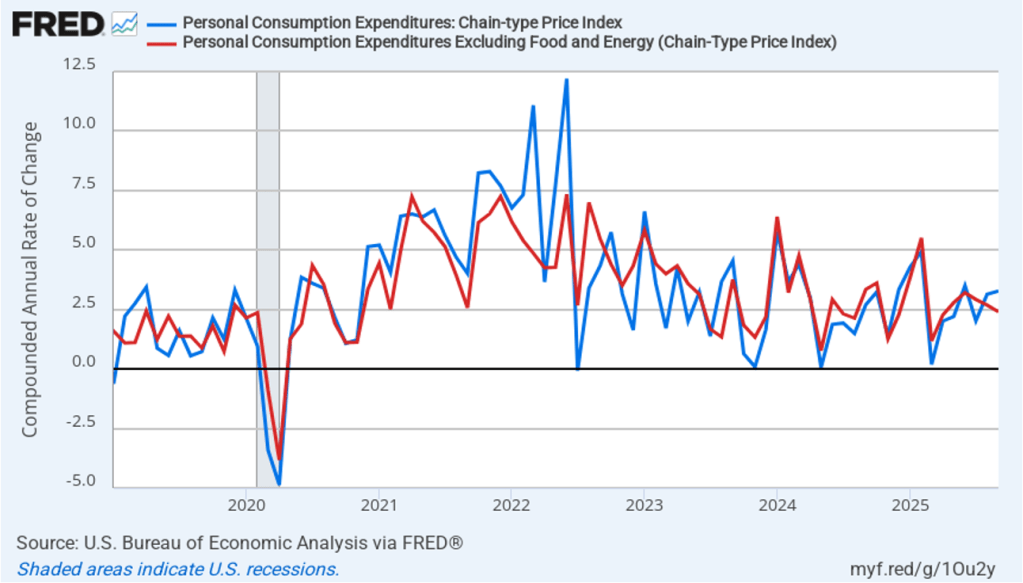
The following figure shows quarterly PCE inflation and quarterly core PCE inflation calculated by compounding the current quarter’s rate over an entire year. Measured this way, headline PCE inflation increased to 2.8 percent in the third quarter of 2025, up from to 2.1 percent in the second quarter. Core PCE inflation increased to 2.9 percent in the third quarter of 2025 from 2.6 percent in the second quarter. Measured this way, both core and headline PCE inflation were well above the Fed’s target.
The relatively strong growth and above-target inflation data from today’s report contrast with last week’s mixed but somewhat weak employment data (which we discuss here) and CPI data that showed inflation significantly slowing (which we discuss here). Note, though, that the employment data were affected by the unusually large decline in federal government employment and the CPI report relied on incomplete data. And, of course, both the employment and GDP data are subject to revision.
In guiding monetary policy, the Federal Reserve’s policymaking Federal Open Market Committee (FOMC) will look for further indications as to whether today’s data showing strong real GDP growth and inflation stuck above the Fed’s target or last week’s data showing both employment growth and inflation slowing are giving a more accurate picture of the state of economy. The FOMC meets next on January 27–28.

Image created by ChatGPT
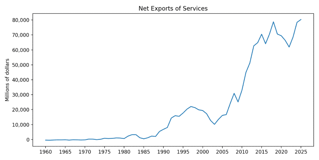
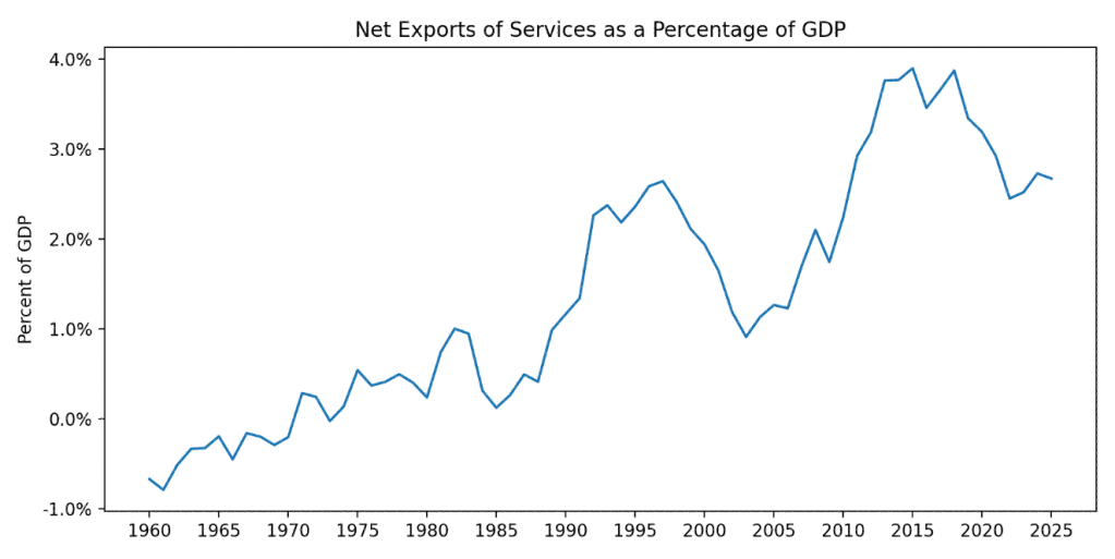
A recent post on the blog of the Federal Reserve Bank of St. Louis reminds us that although the media and some policymakers tend to focus on the fact that the United States typically runs a deficit in trade in goods, it also typically runs a surplus in trade in services. We discuss these points in Economics, Chapter 9, Section 9.1 and Chapter 28, Section 28.1 (Macroeconomics, Chapter 7, Section 7.1 and Chapter 18, Section 18.1, and Microeconomics, Section 9.1). The first of the following figures shows U.S. net exports in services in dollar terms for the period from the first quarter of 1960 through the second quarter of 2025. The second figure show U.S. net exports in services as a percentage of U.S. GDP.
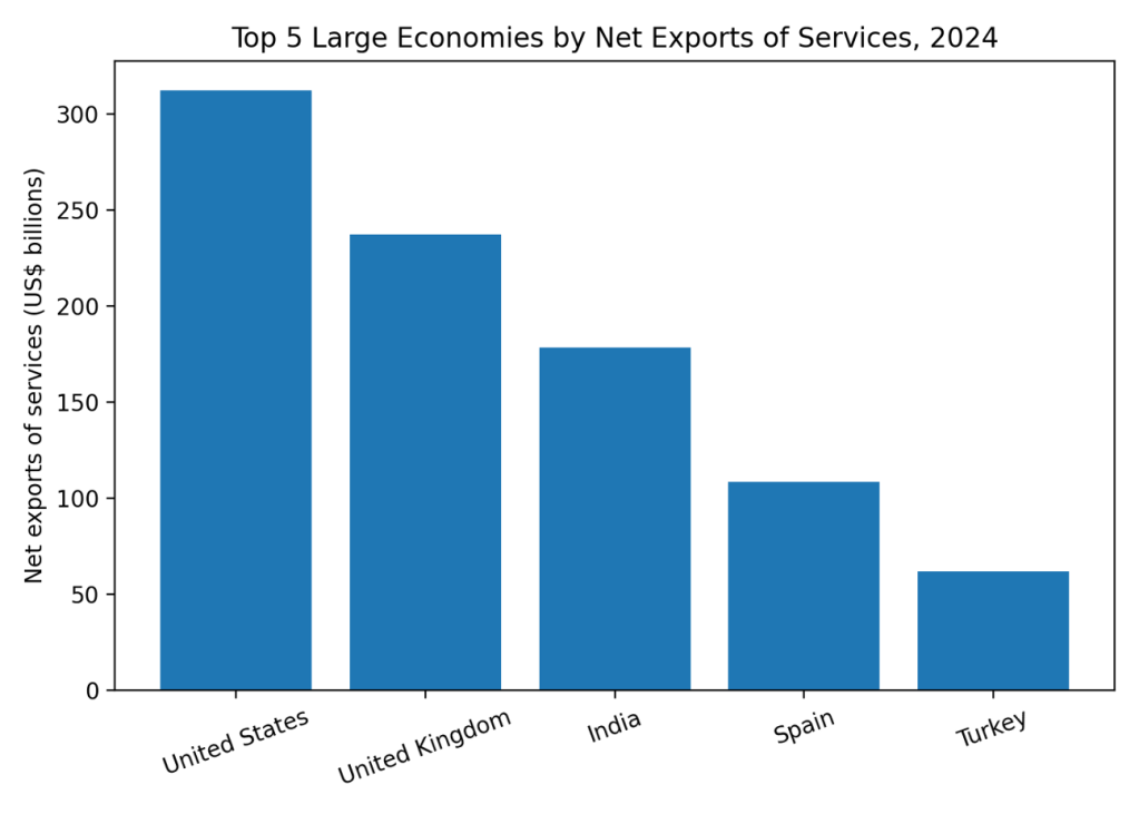
How does the United States compare to other countries? The following figure shows for 2024 the leaders in net exports of services for large economies (those with GDP of $1 trillion or more). The United States has largest value for net exports of services followed by the United Kingdom. China had negative net exports of services in 2024.
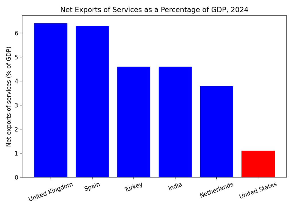
The following figure shows net exports in services as percentage of GDP among large economies. Measured this way, the largest net exporter of services is the United Kingdom, followed by Spain. The United States is included in graph (in red) for comparison and ranks ninth.
The following table from the St. Louis Fed’s blog posts shows the U.S. industries that export the most services.
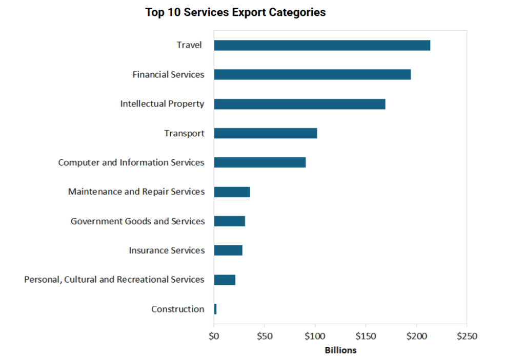
The export of travel services represents largely foreign tourism in the United States. For example, if a family from France visits Walt Disney World in Florida, their spending would be included as an export of travel services.

Image generated by ChatGPT
On Thursday (December 18) the Bureau of Labor Statistics (BLS) released its latest report on the consumer price index (CPI). The federal government shutdown, which lasted from October 1 to November 12, is still affecting the macroeconomic statistics being gathered by the BLS and other agencies. The BLS notes in the report:
“BLS did not collect survey data for October 2025 due to a lapse in appropriations. BLS was unable to retroactively collect these data. For a few indexes, BLS uses nonsurvey data sources instead of survey data to make the index calculations. BLS was able to retroactively acquire most of the nonsurvey data for October. CPI data collection resumed on November 14, 2025.”
The following table from the CPI report gives an indication of how much data that is normally collected wasn’t collected in October or November.

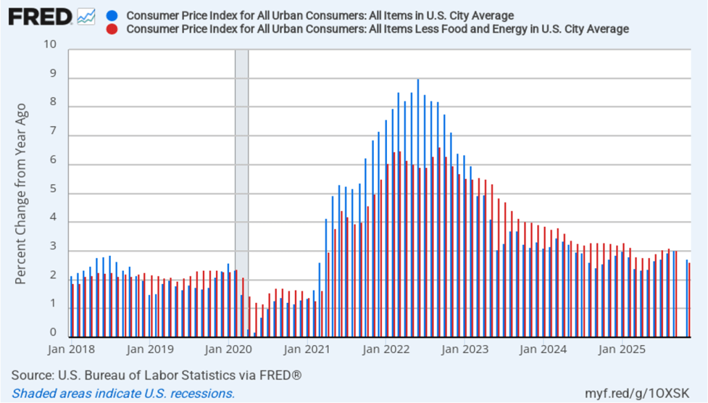
Bearing in mind the missing data, the following figure compares headline CPI inflation (the blue bar) and core CPI inflation (the red bar) as reported in this month’s CPI report.
Economists who were surveyed by Fact Set had forecast that both headline inflation and core inflation would rise to 3.1 percent in November. Economists surveyed by the Wall Street Journal also forecast that headline inflation would rise to 3.1 percent in November, but forecast that core inflation would rise slightly less to 3.0 percent. It’s unclear whether the economists were aware at the time they were surveyed how much data for October and November would be missing from this month’s report.
Because of how much data that is normally collected was missing from the calculations of November’s inflation rate, the results should be treated with caution. The Wall Street Journal quoted an economist at the investment bank UBS as advising: “I think you largely just put this one to the side. Maybe this report gives a minor downward sign for overall inflation, but the vast, vast majority of this is just noise and should be ignored.”
Several economists were concerned about the computation the BLS had to make to deal with the lack of direct data on the price of “shelter.” The price of shelter in the CPI, as explained here, includes both rent paid for an apartment or a house and “owners’ equivalent rent of residences (OER),” which is an estimate of what a house (or apartment) would rent for if the owner were renting it out. OER is included in the CPI to account for the value of the services an owner receives from living in an apartment or house. The following figure shows CPI inflation, measured as the percentage change since the same month in the previous year, leaving out the price of shelter. Measured this way, inflation was 2.6 percent in November, which is slightly lower than the 2.7 percent inflation rate the BLS reported when including all items.

What effect have the tariffs that the Trump administration announced on April 2 had on inflation? (Note that many of the tariff increases announced on April 2 have since been reduced.) The following figure shows 12-month inflation in durable goods—such as furniture, appliances, and cars—which are likely to be affected directly by tariffs, and services, which are less likely to be affected by tariffs. To make recent changes clearer, we look only at the months since January 2022. In November, inflation in durable goods decreased to 1.8 percent from 2.2 percent in September. Inflation in services in November was 3.2 percent, down from 3.6 percent in September. So the upward pressure on goods prices from the tariffs seems to be declining. But, again, missing data makes it’s unclear to what extent November inflation numbers are representative of what’s actually happening currently to prices.

It’s unlikely that this inflation report will have much effect on the views of the members of the Federal Reserve’s policymaking Federal Open Market Committee. In a press conference after the committee’s most recent meeting, Fed Chair Jerome Powell cautioned against drawing firm conclusions from data for October and November:
“I should mention on the data, as long as I’m talking about it, that we’re going to need to be careful in assessing particularly the household survey data. There are very technical reasons about the way data are collected in some of these measures, both in, you know, inflation and in labor—in the labor market so that the data may be distorted. And not just sort of more volatile, but distorted. And that—it’s—and that’s really because data was not collected in October and half of November. So we’re going to get data, but we’re going to have to look at it carefully and with a somewhat skeptical eye by the time of the January meeting ….”

Image created by ChatGPT
Because of the federal government shutdown from October 1 to November 12, the regular release by the Bureau of Labor Statistics (BLS) of its monthly “Employment Situation” report (often called the “jobs report”) has been disrupted. The jobs report usually has two estimates of the change in employment during the month: one estimate from the establishment survey, often referred to as the payroll survey, and one from the household survey. As we discuss in Macroeconomics, Chapter 9, Section 9.1 (Economics, Chapter 19, Section 19.1), many economists and Federal Reserve policymakers believe that employment data from the establishment survey provide a more accurate indicator of the state of the labor market than do the household survey’s employment data and unemployment data. (The groups included in the employment estimates from the two surveys are somewhat different, as we discuss in this post.)
Today, the BLS released a jobs report that has data from the payroll survey for both October and November, but data from the household survey only for November. Because of the government shutdown, the household survey for October wasn’t conducted.
According to the establishment survey, there was a net decrease of 105,000 nonfarm jobs in October and a net increase of 64,000 nonfarm jobs in November. The increase for November was above the increase of 40,000 that economists surveyed by FactSet had forecast. Economists surveyed by the Wall Street Journal had forecast a net increase of 45,000 jobs. The BLS revised downward by a combined 33,000 jobs its previous estimates of employment in August and September. (The BLS notes that: “Monthly revisions result from additional reports received from businesses and government agencies since the last published estimates and from the recalculation of seasonal factors.”)
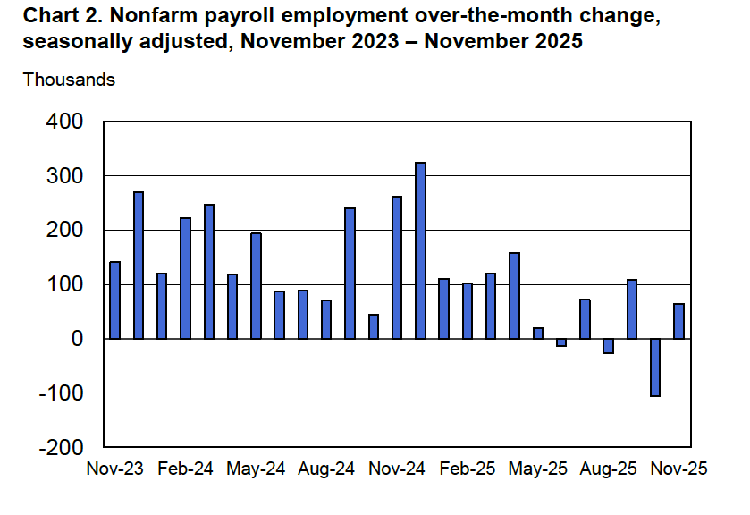
The following figure from the jobs report shows the net change in nonfarm payroll employment for each month in the last two years. The figure illustrates that, as the BLS notes in the report, nonfarm payroll employment “has shown little net change since April.” The Trump administration announced sharp increases in U.S. tariffs on April 2. Media reports indicate that some firms have slowed hiring due to the effects of the tariffs or in anticipation of those effects. In addition, a sharp decline in immigration has slowed growth in the labor force.
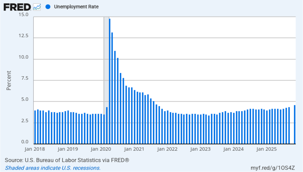
The unemployment rate estimate relies on data collected in the household survey, so there id no unemployment estimate for October. As shown in the following figure, the unemployment rate increased from 4.4 percent in September to 4.6 percent in November, the highest rate since September 2021. The unemployment rate is above the 4.4 percent rate economists surveyed by FactSet had forecast. The unemployment rate had been remarkably stable, staying between 4.0 percent and 4.2 percent in each month from May 2024 to July 2025, before breaking out of that range in August. The Federal Open Market Committee’s current estimate of the natural rate of unemployment—the normal rate of unemployment over the long run—is 4.2 percent. So, unemployment is now well above the natural rate. (We discuss the natural rate of unemployment in Macroeconomics, Chapter 9 and Economics, Chapter 19.)
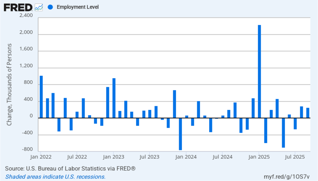
As the following figure shows, the monthly net change in jobs from the household survey moves much more erratically than does the net change in jobs from the establishment survey. As measured by the household survey, there was a net increase of 96,000 jobs from September to November. In the payroll survey, there was a net decrease in of 41,000 jobs from September to November. In any particular month, the story told by the two surveys can be inconsistent. In this case, we are measuring the change in jobs over a two month interval because there is no estimate from the household survey of employment in October. Over that two month period the household survey is showing more strength in the labor market than is the payroll survey. (In this blog post, we discuss the differences between the employment estimates in the two surveys.)
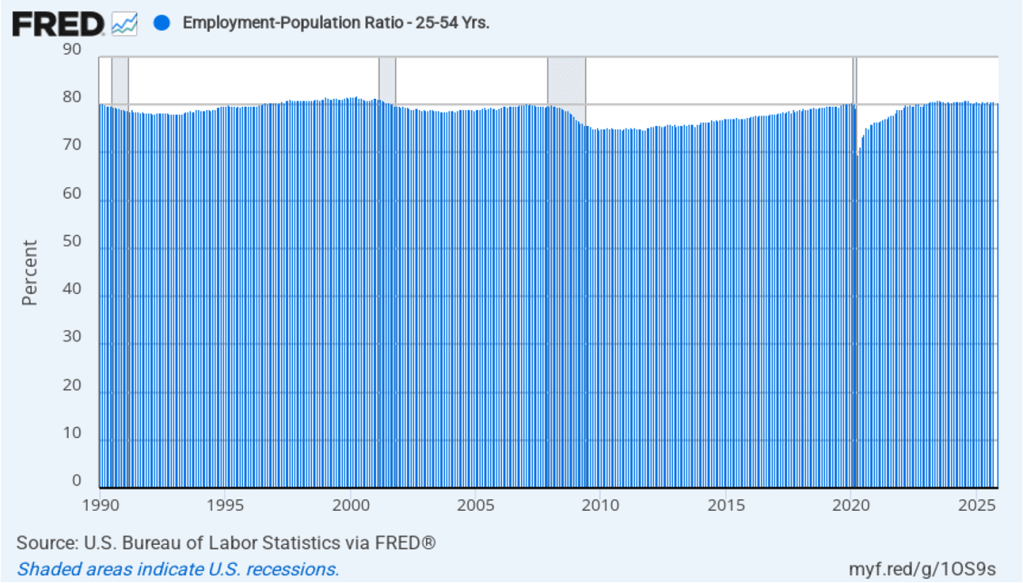
The household survey has another important labor market indicator: the employment-population ratio for prime age workers—those workers aged 25 to 54. In November the ratio was 80.6 percent, down slightly from 80.7 in September. (Again, there is no estimate for October.) The prime-age employment-population ratio is somewhat below the high of 80.9 percent in mid-2024, but is still above what the ratio was in any month during the period from January 2008 to February 2020. The continued high levels of the prime-age employment-population ratio indicates some continuing strength in the labor market.
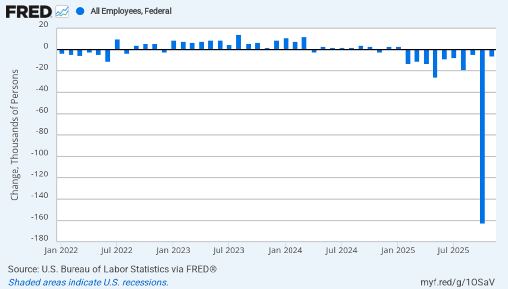
The Trump Administration’s layoffs of some federal government workers are clearly shown in the estimate of total federal employment for October, when many federal government employees exhausted their severance pay. (The BLS notes that: “Employees on paid leave or receiving ongoing severance pay are counted as employed in the establishment survey.”) As the following figure shows, there was a decline federal government employment of 162,000 in October, with an additional decline of 6,000 In November. The total decline since the beginning of February 2025 is 271,000. At this point, we can say that the decline in federal employment has had a significant effect on the overall labor market and may account for some of the rise in the unemployment rate.
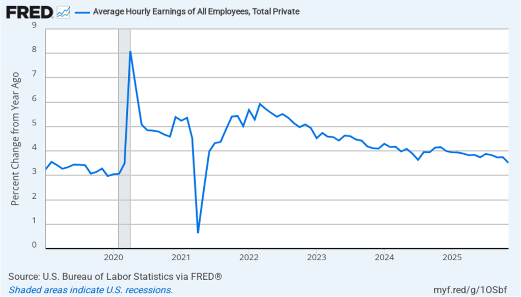
The establishment survey also includes data on average hourly earnings (AHE). As we noted in this post, many economists and policymakers believe the employment cost index (ECI) is a better measure of wage pressures in the economy than is the AHE. The AHE does have the important advantage of being available monthly, whereas the ECI is only available quarterly. The following figure shows the percentage change in the AHE from the same month in the previous year. The AHE increased 3.5 percent in November, down from 3.7 percent in October.
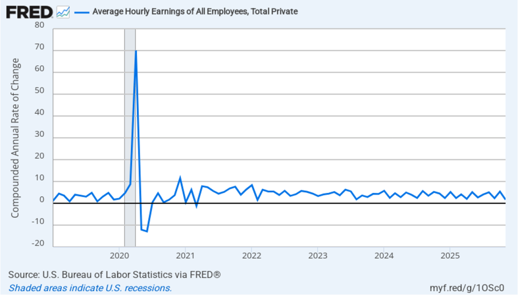
The following figure shows wage inflation calculated by compounding the current month’s rate over an entire year. (The figure above shows what is sometimes called 12-month wage inflation, whereas this figure shows 1-month wage inflation.) One-month wage inflation is much more volatile than 12-month wage inflation—note the very large swings in 1-month wage inflation in April and May 2020 during the business closures caused by the Covid pandemic. In November, the 1-month rate of wage inflation was 1.6 percent, down from 5.4 percent in October. This slowdown in wage growth may be an indication of a weakening labor market. But one month’s data from such a volatile series may not accurately reflect longer-run trends in wage inflation.
What effect might today’s jobs report have on the decisions of the Federal Open Market Committee (FOMC) with respect to setting its target range for the federal funds rate? Today’s jobs report provides a mixed take on the state of the labor market with very slow job growth—although the large decline in federal employment is a confounding factor—a continued high employment-population ratio for prime age workers, and slowing wage growth.
One indication of expectations of future changes in the FOMC’s target for the federal funds rate comes from investors who buy and sell federal funds futures contracts. (We discuss the futures market for federal funds in this blog post.) This morning, investors assigned a 75.6 percent probability to the committee leaving its target range unchanged at 3.50 percent to 3.75 percent at its next meeting on January 27–28. That probability is unchanged from the probability yesterday before the release of the jobs report. Investors apparently don’t see today’s report as providing much new information on the current state of the economy.

Photo from federalreserve.gov
Today’s meeting of the Federal Reserve’s policymaking Federal Open Market Committee (FOMC) had the expected result with the committee deciding to lower its target for the federal funds rate from a range of 3.75 percent to 4.00 percent to a range of 3.50 percent to 3.75 percent—a cut of 25 basis points. The members of the committee voted 9 to 3 in favor of the cut. Fed Governor Stephen Miran voted against the action, preferring to lower the target range for the federal funds rate by 50 basis points. President Austan Goolsbee of the Federal Reserve Bank of Chicago and President Jeffrey Schmid of the Federal Reserve Bank of Kansas City also voted against the action, preferring to leave the target range unchanged.
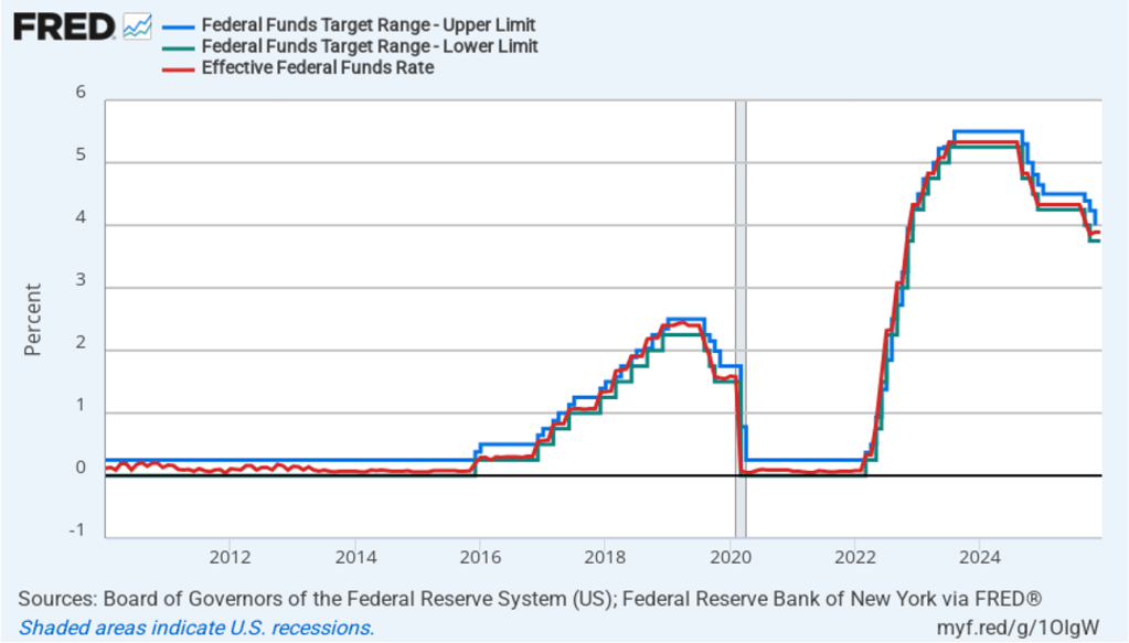
The following figure shows for the period since January 2010, the upper bound (the blue line) and the lower bound (the green line) for the FOMC’s target range for the federal funds rate, as well as the actual values for the federal funds rate (the red line). Note that the Fed has been successful in keeping the value of the federal funds rate in its target range. (We discuss the monetary policy tools the FOMC uses to maintain the federal funds rate within its target range in Macroeconomics, Chapter 15, Section 15.2 (Economics, Chapter 25, Section 25.2).)
After the meeting, the committee also released a “Summary of Economic Projections” (SEP)—as it typically does after its March, June, September, and December meetings. The SEP presents median values of the 19 committee members’ forecasts of key economic variables. The values are summarized in the following table, reproduced from the release. (Note that only 5 of the district bank presidents vote at FOMC meetings, although all 12 presidents participate in the discussions and prepare forecasts for the SEP.)
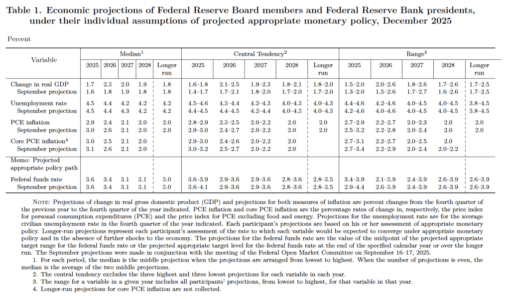
There are several aspects of these forecasts worth noting:
Prior to the meeting there was much discussion in the business press and among investment analysts about the dot plot, shown below. Each dot in the plot represents the projection of an individual committee member. (The committee doesn’t disclose which member is associated with which dot.) Note that there are 19 dots, representing the 7 members of the Fed’s Board of Governors and all 12 presidents of the Fed’s district banks.
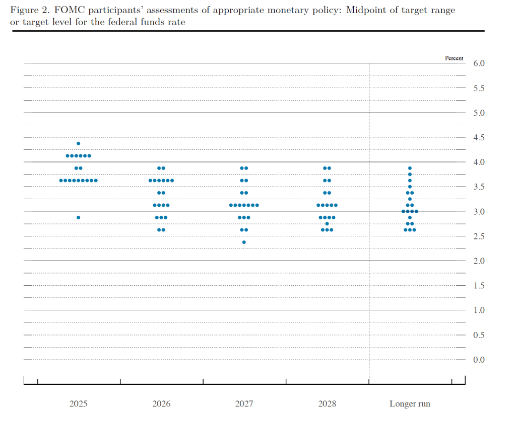
The plots on the far left of the figure represent the projections by the 19 members of the value of the federal funds rate at the end of 2025. The fact that several members of the committee preferred that the federal funds rate end 2025 above 4 percent—in other words higher than it will be following the vote at today’s meeting—indicates that several non-voting district bank presidents, beyond Goolsbee and Schmid, would have preferred to not cut the target range. The plots on the far right of the figure indicate that there is substantial disagreement among comittee members as to what the long-run value of the federal funds rate—the so-called neutral rate—should be.
During his press conference following the meeting, Powell indicated that the increase in inflation in recent months was largely due to the effects of the increase in tariffs on goods prices. Powell indicated that committee members expect that the tariff increases will cause a one-time increase in the price level, rather than causing a long-term increase in the inflation rate. Powell also noted the recent slow growth in employment, which he noted might actually be negative once the Bureau of Labor Statistics revises the data for recent months. This slow growth indicated that the risk of unemployment increasing was greater than the risk of inflation increasing. As a result, he said that the “balance of risks” caused the committee to believe that cutting the target for the federal funds rate was warranted to avoid the possibility of a significant rise in the unemployment rate.
The next FOMC meeting is on January 27–28. By that time a significant amount of new macroeconomic data, which has not been available because of the government shutdown, will have been released. It also seems likely that President Trump will have named the person he intends to nominate to succeed Powell as Fed chair when Powell’s term ends on May 15, 2026. (Powel’s term on the Board doesn’t end until January 31, 2028, although he declined at the press conference to say whether he will serve out the remainder of his term on the Board after he steps down as chair.) In addition, it’s possible that by the time of the next meeting the Supreme Court will have ruled on whether President Trump can legally remove Governor Lisa Cook from the Board and on whether President Trump’s tariff increases this year are Constitutional.

Image created by ChatGPT
Today (December 5), the Bureau of Economic Analysis (BEA) released monthly data on the personal consumption expenditures (PCE) price index for September as part of its “Personal Income and Outlays” report. Release of the report was delayed by the federal government shutdown.
The following figure shows headline PCE inflation (the blue line) and core PCE inflation (the red line)—which excludes energy and food prices—with inflation measured as the percentage change in the PCE from the same month in the previous year. In September, headline PCE inflation was 2.8 percent, up slightly from 2.7 percent in August. Core PCE inflation in September was also 2.8 percent, down slightly from 2.9 percent in August. Both headline and core PCE inflation were equal to the forecast of economists surveyed.
The following figure shows headline PCE inflation and core PCE inflation calculated by compounding the current month’s rate over an entire year. (The figure above shows what is sometimes called 12-month inflation, while the figure below shows 1-month inflation.) Measured this way, headline PCE inflation increased from 3.1 percent in August to 3.3 percent in September. Core PCE inflation declined from 2.7 percent in August to 2.4 percent in September. So, both 1-month and 12-month PCE inflation are telling the same story of inflation somewhat above the Fed’s target. The usual caution applies that 1-month inflation figures are volatile (as can be seen in the figure). In addition, these data are for September and likely don’t fully reflect the situation nearly two months later.
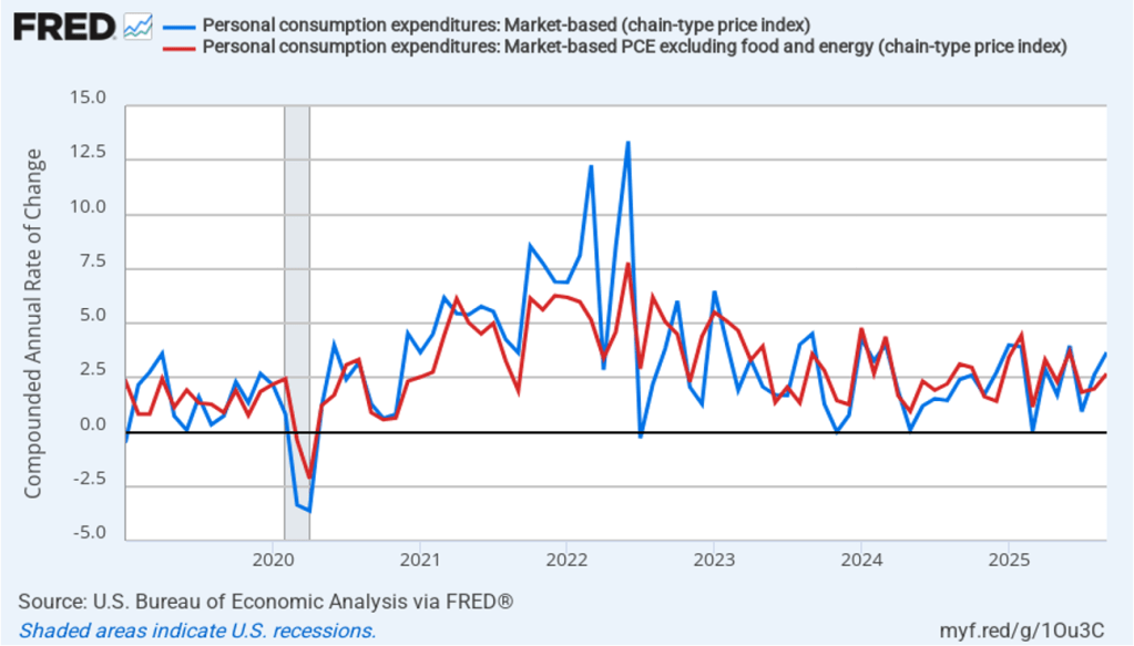
Fed Chair Jerome Powell has frequently mentioned that inflation in non-market services can skew PCE inflation. Non-market services are services whose prices the BEA imputes rather than measures directly. For instance, the BEA assumes that prices of financial services—such as brokerage fees—vary with the prices of financial assets. So that if stock prices fall, the prices of financial services included in the PCE price index also fall. Powell has argued that these imputed prices “don’t really tell us much about … tightness in the economy. They don’t really reflect that.” The following figure shows 12-month headline inflation (the blue line) and 12-month core inflation (the red line) for market-based PCE. (The BEA explains the market-based PCE measure here.)
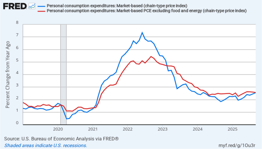
Headline market-based PCE inflation was 2.6 percent in September, up from 2.4 percent in August. Core market-based PCE inflation was 2.6 percent in September, unchanged from August. So, both market-based measures show inflation as stable but above the Fed’s 2 percent target.
In the following figure, we look at 1-month inflation using these measures. One-month headline market-based inflation increase sharply to 3.7 percent in September from 2.6 percent in August. One-month core market-based inflation increased to 2.7 percent in September from 2.0 percent in August. As the figure shows, the 1-month inflation rates are more volatile than the 12-month rates, which is why the Fed relies on the 12-month rates when gauging how close it is coming to hitting its target inflation rate.
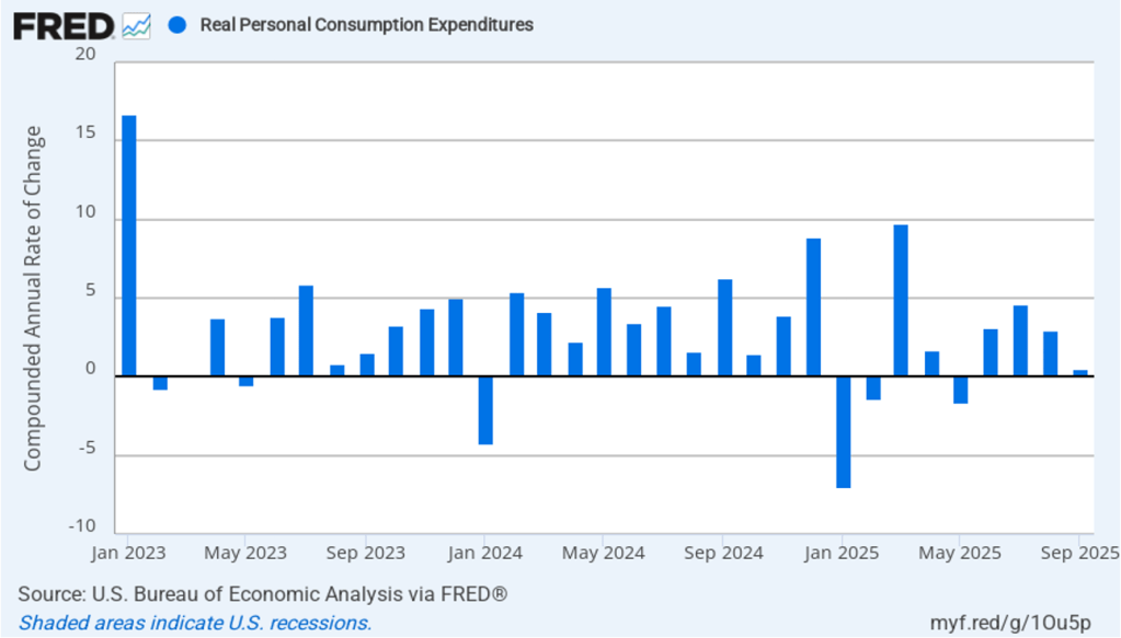
Data on real personal consumption expenditures were also included in this report. The following figure shows compound annual rates of growth of real real personal consumptions expenditures for each month since January 2023. Measured this way, the growth in real personal consumptions expenditures slowed sharply in September to 0.5 percent from 3.0 percent in August.
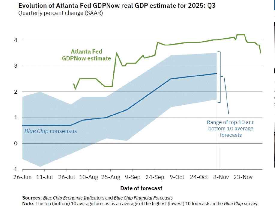
Does the slowing in consumptions spending indicate that real GDP may have also grown slowly in the third quarter of 2025? Economists at the Federal Reserve Bank of Atlanta prepare nowcasts of real GDP. A nowcast is a forecast that incorporates all the information available on a certain date about the components of spending that are included in GDP. The Atlanta Fed calls its nowcast GDPNow. As the following figure from the Atlanta Fed website shows, today the GDPNow forecast—taking into account today’s data on real personal consumption expenditures—is for real GDP to grow at an annual rate of 3.5 percent in the third quarter, which reflects continuing strong growth in other measures of output.
In a number of earlier blog posts, we discussed the policy dilemma facing the Fed. Despite the Atlanta Fed’s robust estimate of real GDP growth, there are some indications that the labor market may be weakening. For instance, earlier this week ADP estimated that private sector employment declined by 32,000 jobs in November. (We discuss ADP’s job estimates in this blog post.) As the Fed’s policy-making Federal Open Market Committee (FOMC) prepares for its next meeting on December 9–10, it has to balance guarding against a potential decline in employment with concern that inflation has not yet returned to the Fed’s 2 percent annual target.
If the committee decides that inflation is the larger concern, it is likely to leave its target range for the federal funds rate unchanged. If it decides that weakness in the labor market is the larger concern, it is likely to reduce it target range by 0.25 percentage point (25 basis points). Statements by FOMC members indicate that opinion on the committee is divided. In addition, the Trump administration has brought pressure on the committee to cut its target rate.
One indication of expectations of future changes in the FOMC’s target for the federal funds rate comes from investors who buy and sell federal funds futures contracts. (We discuss the futures market for federal funds in this blog post.) Investors’ expectations have been unusually volatile during the past two months as new macroeconomic data or new remarks by FOMC members have caused swings in the probability that investors assign to the committee cutting the target range.
As of this afternoon, investors assigned a 87.2 percent probability to the committee cutting its target range for the federal funds rate by 25 basis points to 3.50 percent to 3.75 percent at its December meeting. At the December meeting the committee will also release its Summary of Economic Projections (SEP) giving members forecasts of future values of the inflation rate, the unemployment rate, the federal funds rate, and the growth rate of real GDP. The SEP, along with Fed Chair Powell’s remarks at his press conference following the meeting, should provide additional information on the monetary policy path the committee intends to follow in the coming months.


Image generated by ChatGPT
A perennial media story this time of year looks at whether a Thanksgiving turkey dinner costs more or less than last year. Not too surprisingly, the answer depends on what side dishes you serve with the turkey. Deloitte provides tax, consulting, and other services to businesses. Their calculation of the cost of a Thanksgiving dinner over the past three years can be found here.
The following image shows the food that they include in their cost calculation. For that particular Thanksgiving dinner, the cost is slightly higher than in 2024, although slightly lower than in 2023.
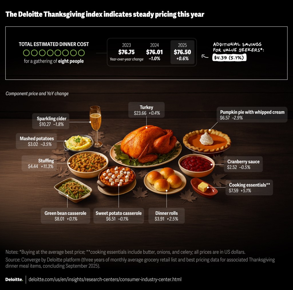
Image from deloitte.com
The following image from the American Farm Bureau Federation, a lobbying organization for U.S. farmers, shows the food they include in their calculation of the cost of a Thanksgiving dinner.
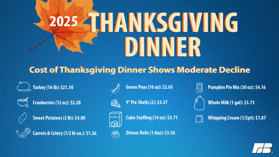
Image from fb.org
For a Thanksgiving dinner with those side dishes, the price is about 5 percent lower this year than last year.
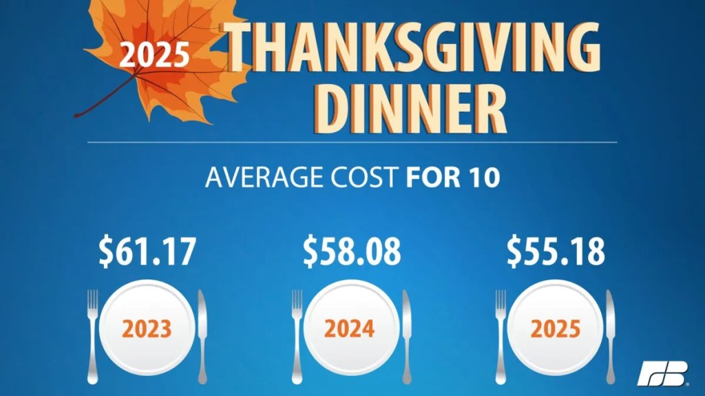
Image from fb.org
Note that the two estimates differ in the cost of the turkey. It’s not clear whether the difference is due to the size of the turkey or to differences in the price of the turkey. Related point: The Bureau of Labor Statistics (BLS) stopped collecting data on retail turkey prices in February 2020, at the start of the pandemic, and never resumed collecting them. Here’s the link to the BLS retail turkey price series on FRED. The series begins in January 1980 and ends in February 2020.
Justin Fox, in a column on bloomberg.com, notes that demand for turkey has been declining in recent years. The following figure uses data on turkey consumption per capita from the U.S. Department of Agriculture.
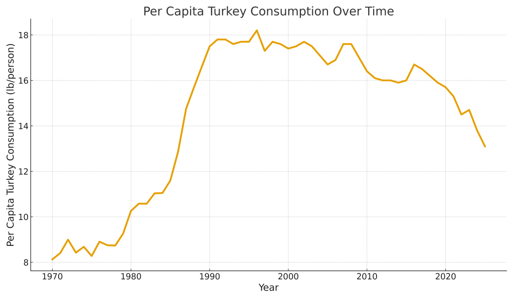
Turkey consumption peaked at 18.2 pounds per person in 1996 and has fallen to an estimated 13.1 pounds per person in 2025—a decline of about 28 percent. Is this decline an indication that people have moved away from eating turkey for Thanksgiving? Fox argues that it likely doesn’t. Note the rapid rise of turkey consumption between 1980 and 1990. Fox believes the surge in consumption was due to “both chicken and turkey [consumption increasing] as health concerns led many Americans to shun red meat starting in the late 1970s ….” In recent years, though, “red-meat consumption has steadied … chicken consumption has continued to rise, and turkey is losing out. Maybe people just don’t like how it tastes.” Glenn and Tony agree that, alas, turkey is often dry—although, admittedly, skilled cooks claim that it isn’t dry when prepared properly.
So, turkey may be holding its own at the heart of Thanksgiving dinners, but seems to be struggling to get on the menu during the rest of the year.
