Supports:Microeconomics and Economics, Chapter 15, Section 15.5, and Essentials of Economics, Chapter 10, Section 10.5
Image generated by ChatGTP-4o
A national provider of cable television and internet service has been frequently criticized by customers on social media for using the following business strategy: The company raises its prices every six to nine months. Any subscriber who calls to complain is offered a discount off of the price increase. Analyze how this strategy can be profit mazimizing for the company.
Step 1: Review the chapter material. This problem is about firms using price discrimination, so you may want to review Chapter 15, Sections 15.5
Step 2: Answer the question by explaining how the cable company is using price discrimination to increase its profit. Price discrimination involves charging different prices to different customers for the same good or service when the price difference isn’t due to differences in cost. Firms who able to price discriminate increase their profits by doing so.
We’ve seen that there are three requirements for a firm to practice price discrimination: 1) The firm must possess market power, 2) some of the firm’s customers much have a greater willingness to pay for the product than do other customers, and 3) the firm must be able to segment the market to keep customers who buy the product at the low price from reselling it. Cable companies can meet all three requirements. Cable firms possess market power—they aren’t perfect competitors. Some customers have a higher willingness than other customers to pay for cable service. In fact, many people have become cable cutters and prefer to stream content rather than watch programs on cable. Finally, someone who receives a lower-priced cable subscription can’t resell it.
To increase profit by price discrimination, a firm needs to charger a higher price to customers with a lower price elasticity of demand, and a lower price to customers with a higher price elasticity of demand. People who call up to complain about an increase in the price of a cable subscription are likely to be more price sensitive—and, therefore, more likely to switch to a competing cable company or to cut the cable and switch to streaming—than are people who don’t complain about the increase in the price of a subscription. In other words, the complainers have a higher price elasticity of demand than do the non-complainers and receive a lower price. We can conclude that this business strategy is an example of price discrimination and will increase the profit of the cable company that uses it.
Supports:Money, Banking, and the Financial System, Chapter 3, Section 3.5
Image generated by ChatGTP-4o
The 30-year U.S. Treasury bond has the longest maturity available on a bond issued by the U.S. government. Some other governments have issued century bonds, which are bonds that don’t mature for 100 years. Bonds with maturities longer than 30 years are sometimes called ultra-long-term bonds. For example, in June 2020 the government of Austria issued a bond that will mature in June 2120. The bond has a par value of €100 and a coupon rate of 0.85%, which seems low but was high in comparison with the yields on other European government bonds at the time. For example, the yield on the 10-year German government bond was negative from April 2019 through January 2021.
Today (April 25), in a newsletter from the Wall Street Journal, Spencer Jakab noted that: “With a little over 95 years remaining, those [Austrian century] bonds now fetch 35 cents on the euro. Investors aren’t worried about being repaid ….”
a. What does Jakab mean that the “bonds now fetch 35 cents on the euro”?
b. If the investors aren’t worried about the Austrian government making coupon or principal payments on the bond, why do the bonds fetch only 35 cents on the euro?
Solving the Problem Step 1: Review the chapter material. This problem is about the relationship between the interest-rate risk on a bond and the bond’s maturity, so you may want to review Money, Banking, and the Financial System, Chapter 3, Section 3.5, “Interest Rates and Rates of Return.”
Step 2: Answer part a. by explaining what Jakab means by writing that Austrian century bonds that mature in 2120 now fetch “35 cents on the euro.” The bonds have a par value (or face value) of €100. By “35 cents on the euro,” Jakab must mean that the current price the bonds are trading at is €35.
Step 3: Answer part b. by explaining why the market price of these Austrian century bonds has declined by 65% from their par value even though the bonds have low default risk. As we discuss in this section of the textbook, long-term bonds have substantial interest-rate risk—the risk that the price of the bond will fluctuate in response to changes in market interest rates—even if they have very low default risk—the risk that an investor won’t receive the coupon and principal payments on the bond. As Table 3.2 in this section shows, the longer the maturity of a bond, the greater the interest-rate risk. As market interest rates on other government bonds have risen, the yield on the Austrian century bonds has also had to rise for investors to be willing to buy these bonds. With a fixed coupon rate of 0.85%, the only way for the yield to rise is for the price of the bonds to fall. Given the very long maturity of these bonds, the price has had to fall by 65% from its par value to make the yield on the bonds competitive with other government bonds.
Supports:Microeconomics and Economics, Chapter 6, and Essentials of Economics, Chapter 7, Section 7.5-7.7
ChatGTP-4o image of cars in the Lincoln Tunnel, which connects New Jersey with midtown Manhattan.
In January 2025, New York City began enforcing congestion pricing in the borough of Manhattan south of 60th Street—the congestion relief zone. The Metropolitan Transportation Authority (MTA) in New York collects a toll from a vehicle entering that zone either automatically using the vehicle’s E-ZPass transponder or by reading the vehicle’s license plate and mailing a bill to the vehicle’s owner. Nobel Laureate William Vickrey of Columbia University first proposed congestion pricing in the 1950s as a way to deal with the negative externalities from traffic congestion. Congestion pricing acts as a Pigovian tax that internalizes the external costs drivers generate by using streets in congested areas. (We discuss Pigovian taxes in Microeconomics and Economics, Chapter 5, Section 5.3, and in Essentials of Economics, Chapter 4, Section 4.3.)
The New York City congestion toll is somewhat complex, varying according to the type of vehicle and how the vehicle enters the area in which the toll applies. The congestion toll fora car entering Manhattan through the Lincoln Tunnel on a weekday between 5 am and 9 pm is $6.00 on top of the existing toll of $16.06. In January 2025, the volume of cars driving through the Lincoln Tunnel declined by 8 percent during the weekday hours of 5 am to 9 pm. According to an article in Crain’s New York Business, the number of vehicles entering the congestion relief zone compared with the same month in the previous year declined by 8 percent in January, 12 percent in February, and 13 percent in March.
From the information given, can we determine the price elasticity of demand for entering Manhattan by driving though the Lincoln Tunnel during weekdays from 5am to 9am? Briefly explain.
Suppose someone makes the following claim: “Because the quantity of cars using the Lincoln Tunnel has declined by 8 percent, we know that the MTA must have collected less revenue from cars using the tunnel than before the congestion toll was imposed.” Briefly explain whether you agree.
Is the pattern of increasing percentage declines in vehicle traffic in the congestion relief zone each month from January to March what we would expect? Be sure your answer refers to concepts related to the price elasticity of demand.
Step 1: Review the chapter material. This problem is about the price elasticity of demand, so you may want to review Chapter 6, Sections 6.1-6.4.
Step 2: Answer part (a) by explaining whether from the information given we can determine the price elasticity of demand for entering Manhattan by driving through the Lincoln Tunnel. We do have sufficient information to determine the price elasticity, provided that nothing else that would affect the demand for driving through the Lincoln Tunnel changed during January. We’re told the percentage change in the quantity demand, so we need only to calculate the percentage change in the price to determine the price elasticity. The change in the price is the $6 congestion toll. The average of the price before and the price after the toll is imposed is ($16.06 + $22.06) = $19.06. Therefore, the percentage change in the price is ($6/$19.06) × 100 = 31.5 percent. The price elasticity of demand is equal to the percentage change in quantity dmanded divided by the percentage change in price: –6%/31.5% = –0.3. Because this value is less than 1 in absolute value, we can conclude that the demand for driving through the Lincoln Tunnel is price inelastic.
Step 3: Answer part (b) by explaining whether because the quantity of cars driving through the Lincoln Tunnel has declined the MTA must have collected less revenue from cars using the tunnel. As shown in Section 6.3 of the textbook, total revenue received will fall after a price increase only if demand is price elastic. In this case, demand is price inelastic, so the total revenue the MTA collects from cars using the Lincoln Tunnel will rise, not fall.
Step 3: Answer part (c) by explaining whether the pattern of increasing percentage declines in vehicle traffic in the congestion relief zone is one we would expect. In Section 6.2, we see that the passage of time is one of the determinants of the price elasticity of demand. The more time that passes, the more price elastic the demand for a product becomes. In other words, the longer the time that people have to adjust to the congestion toll—by, for instance, taking a bus rather than driving through the Lincoln Tunnel in a car—the more likely it is that people will decide not to drive into the congestion relief zone. So, it is not surprising that the number of vehicles entering the congestion relief zone declined by a greater percentage each month from January to March.
Supports:Microeconomics and Economics, Chapter 11, Section 11.5, and Essentials of Economics, Chapter 8, Section 8.5
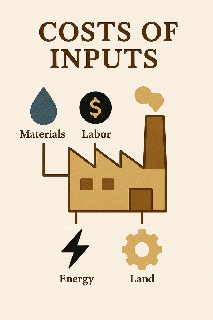
Image generated by ChatGTP-4o showing the costs of inputs to a factory.
Mickey, the Econ Pup, sometimes struggles with drawing and interpreting cost curves. Examine the cost curves shown in images a. and b. and let Mickey know if you find any errors.
a.
b.
Solving the Problem Step 1: Review the chapter material. This problem is about drawing and interpreting cost curves, so you may want to review Chapter 11, Section 11.5, “Graphing Cost Curves.”
Step 2: Answer part a. by explaining whether there are any errors in the cost curves shown in the image in a. No wonder Mickey is confused! This figure has multiple errors:
It’s an error to have the ATC and AVC curves cross. The unlabeled curve at the bottom is supposed to be AFC. We know that if a firm has fixed costs, then the ATC and AVC curves will get closer and closer as the quantity increases and AFC becomes smaller and smaller. But because AFC will never decline to zero, ATC and AVC can’t be equal at any quantity.
The second error is related to the first error. We know that the MC and ATC curves should intersect at the quantity at which ATC is at a minimum. In this figure, the MC curve intersects the ATC curve at a quantity that is larger than the quantity at which ATC recaches a minimum.
The third error is related to the first two errors. The relationship between the three average cost curves should be ATC = AVC + AFC at every quantity. In this figure the relationship doesn’t hold at any quantity.
Finally, there is a dotted line from the point where the (unlabeled) AFC curve intersects with the MC curve down to the Q-axis. But that point has no economic significance.
Step 3: Answer part b. by explaining whether there are any errors in the cost curves shown in image b. Mickey can rest easy with these cost curve because, although the figure seems to be only partially finished, all of the cost curves are correctly drawn. The MC curve correctly intersects the AVC curve at the quantity at which the AVC curve is at a minimum. The instructor could finish the figure by labeling the bottom curve as AFC and by drawing an ATC curve above the AVC curve, with the ATC curve intersecting the MC curve at the quantity at which the ATC curve is at a minimum.
Image generated by ChatGTP-4o of new cars on a dealer’s lot.
This afternoon (April 2), President Donald Trump announced a sweeping increase in tariff rates on imported goods. The increases were by far the largest since the Smoot-Hawley Tariff of 1930. The United States will impose 10 percent across-the-board tariff on all imports, with higher tariffs being imposed on individual countries. Taking into account earlier tariffs, Chinese imports will be subject to a 54 percent tariff. Imports from Vietnam will be subject to a 46 percent tariff, and imports from the countries in the European Union will be subject to a 20 percent tariff.
President Trump’s objectives in imposing the tariffs aren’t entirely clear because he and his advisers have emphasized different goals at different times. The most common objectives the president and his advisers have offered for the tariff increases are these three:
To increase the size of the U.S. manufacturing sector by raising the prices of imported manufactured goods.
To retaliate against barriers that other countries have raised against U.S. exports.
To raise revenue for the federal government.
The effects of the tariffs on the U.S. economy depend in part on whether foreign countries retaliate by raising their tariffs on imports from the United States and on whether, in the future, the president reduces tariffs in exchange for other countries reducing barriers to U.S. imports. For a background discussion of tariffs, see this post. Glenn and Tony discuss tariffs in this podcast, which was recorded on Friday afternoon (March 28). A discussion of the Smoot-Hawley Tariff can be found here.
The following Solved Problem looks at one aspect of the effects of a tariff increase.
Supports:Microeconomics and Economics, Chapter 6, Section 6.3.
Nearly every automobile assembled in the United States contains at least some imported parts. An article on axis.com made the following statement about the effect on U.S. automobile manufacturers of an increase in the tariff on imported auto parts: “If car prices [in the United States] go up, Americans will buy fewer of them, meaning less revenue ….” What assumption is the author of this article making about the demand for new automobiles in the United States?
Solving the Problem
Step 1: Review the chapter material. This problem is about the effect of price increases on a firm’s revenue, so you may want to review the section “The Relationship between Price Elasticity of Demand and Total Revenue.”
Step 2: Answer the question by explaining what must be true of the demand for new automobiles in the United States if an increase in automobile prices results in a decline in the revenue received by automobile producers. This section of Chapter 6 explains how the price elasticity of demand affects the revenue a firm receives following a price increase. A price increase, holding everything else constant that affects the demand for a good, always causes a decline in the quantity demanded. If demand is price inelastic, an increase in price will result in an increase in revenue because the percentage decline in quantity demanded will be smaller than the percentage increase in the price. If demand is price elastic, an increase in price will result in a decrease in revenue because the percentage decline in the quantity demanded will be larger than the percentage increase in price. We can conclude that the author of the article must be assuming that the demand for new automobiles in the United States is price elastic.
A column in the New York Times made the following observations:
“The greenback has been climbing since Trump’s victory, a potential drag on multinationals’ profits. Elsewhere, the yield on the closely watched 10-year Treasury note ticked higher again on Tuesday ….”
What is a “greenback”? What does it mean to say that the greenback has been “climbing”? Climbing relative to what?
Is there a connection between the interest rate on the 10-year U.S. Treasury note increasing and the value of the greenback increasing? Briefly explain.
Why would an increase in the value of the greenback be a potential drag on the profits of U.S.-based multinationals?
Solving the Problem
Step 1: Review the chapter material. This problem is about the effect of changes in the ex-change rate, so you may want to review the section “The Foreign Exchange Market and Exchange Rates.”
Step 2: Answer part (a) by explaining what a greenback is and what it means to say that the greenback is climbing. “Greenback” is a slang term for the U.S. dollar because the back of U.S. currency is printed in green ink. The “greenback climbing” means that the U.S. dollar is increasing in value relative to other currencies—in other words, the exchange rate is increasing.
Step 3: Answer part (b) by explaining whether there is a connection between the value of the U.S. dollar increasing as the interest rate on the 10-year U.S. Treasury note is increasing. There is a connection: Higher interest rates in the United States will make investing in U.S. financial securities, such as Treasury notes, more attractive to foreign investors. Foreign investors will increase their demand for dollars, increasing the equilibrium exchange rate.
Step 3: Answer part (c) by explaining why an increase in the value of the greenback will affect the profits of U.S. multinational corporations. A U.S. multinational firm, such as Microsoft or Apple, will have operations in other countries. When, for instance, Microsoft sells access to its Office Suite to customers in France of Germany, the customers pay in euros. If the value of the dollar has risen in exchange for euros, when Microsoft converts the euros into dollars it receives fewer dollars, thereby reducing its profits.
Supports: Macroeconomics, Microeconomics, Economics, and Essentials of Economics, Chapter 3, Section 3.1.
Photo from theathletic.com
Caitlin Clark had a sensational college career at the University of Iowa, being named National Player of the Year in her junior and senior years. She was chosen first by the Indiana Fever in the 2024 Women’s National Basketball Association (WNBA) draft of college players. Her popularity drew large crowds to both her home and away games during the 2024 season.
In 2023, the Indiana Fever sold an average of 4,067 tickets to its home games. In 2024, with Clark on the team, the Fever sold an average of 17,036 to its home games. The average price the Fever charged per ticket increased from $60 in 2023 to $110 in 2024. As an article on theathletic.com put it: “Despite the higher price point, even more tickets were sold [by the Fever] this year.”
Can we conclude from this information that Caitlin Clark is so popular that the demance curve for Fever tickets is upward sloping? Briefly explain.
Solving the Problem Step 1: Review the chapter material. This problem is about the effect of a price change on the quantity demand of a good or service, so you may want to review Chapter 3, Section 3.1, “The Demand Side of the Market.”
Step 2: Answer the question by explaining whether it’s likely that the demand curve for tickets to Fever games is upward sloping. It’s unlikely that the demand curve for tickets to Fever games is upward sloping. The law of demand states that, holding everything else constant, when the price of a product rises, the quantity demanded of the product will decrease. When the Fever raised ticket prices from $60 in 2023 to $100 in 2024, we would expect the result to be a movement up the demand curve for tickets, resulting in fewer tickets sold, provided that everything else that would affect the demand for tickets was constant between 2023 and 2024. But everything wasn’t constant because the Fever had Clark on the team in 2024 but not in 2023. Her popularity increased the demand for tickets, shifting the demand curve to the right. In other words, the shift in demand allowed the Fever to sell more tickets at a higher price—moving from a price of $60 and a quantity of 4,067 on the 2023 demand curve to a price of $110 and a quantity of 17,036 on the 2024 demand curve.
Supports: Macroeconomics, Chapter 9,Economics, Chapter 19, and Essentials of Economics, Chapter 13.
Image generated by GTP-4o.
In its “Employment Situation” report for July 2024, the Bureau of Labor Statistics (BLS) stated that according to the household survey the total number of people employed, the total number of people unemployed, and the unemployment rate all increased. Would we expect this result to always hold? That is, in a month in which both the total number of people employed and the total number of people unemployed increased will the unemployment rate always increase? Briefly explain.
Solving the Problem Step 1: Review the chapter material. This problem is about calculating the unemployment rate, so you may want to review Chapter 9, Section 9.1, “Measuring the Unemployment Rate, the Labor Force Participation Rate, and the Employment-Population Ratio.”
Step 2: Answer the question by explaining whether we can be certain what happens to the unemployment rate in a month in which both the total number of people employed and the total number of people unemployed increased. The unemployment rate is equal to the number of people unemployed divided by the number of people in the labor force (multiplied by 100). The labor force equals the sum of the number of people employed and the number of people unemployed.
Suppose, for example, that the unemployment rate in the previous month was 4 percent. If both the number of people employed and the number of people unemployed increase, the unemployment rate will increase if the increase in the number of people unemployed as a percentage of the increase in the labor force is greater than 4 percent. The unemployment rate will decrease if the increase in the number of people unemployed as a percentage of the increase in the labor force is less than 4 percent.
Consider a simple numerical example. Suppose that in the previous month there were 96 people employed and 4 people unemployed. In that case, the unemployment rate will be (4/(96 + 4)) x 100 = 4.0%.
Suppose that during the month the number of people employed increases by 30 and the number of people unemployed increases by 1. In that case, there are now 126 people employed and 5 people unemployed. The unemployment rate will have fallen from 4.0% to (5/(126 + 5)) x 100 = 3.8%.
Now suppose that the number of people employed increased by 30 and the number of people unemployed increases by 3. The unemployment will have risen from 4.0% to (7/(126 + 7)) x 100 = 5.3%.
We can conclude that what happened in July 2024 need not always happen. If both the total number of people employed and the total number of people unemployed increased during a given month, we can’t be sure whether the unemployment rate has increased or decreased.
Chicago Cubs Hall of Fame shortstop Ernie Banks was known for saying “It’s a great day for baseball. Let’s play two!” (Photo from the Baseball Hall of Fame)
First Solved Problem: Exchange Rates and Tourism
Supports: Macroeconomics, Chapter 18, Sections 18.2 and 18.6; and Economics, Chapter 28, Sections 28.2 and 28.6.
The headline of an article on nbcnews.com is: “The Fed May Soon Cut Interest Rates. That Could Make Your Next Trip Abroad More Expensive.”
Briefly explain the difference between a “strong dollar” and a “weak dollar.”
If you are going to spend two weeks on vacation in France, would you prefer that the dollar be strong or weak during that time? Briefly explain.
Briefly explain the connection between Federal Reserve monetary policy and the exchange rate between the U.S. dollar and other currencies.
Use your answers to parts a., b., and c. to explain what the headline means.
Solving the Problem
Step 1: Review the chapter material. This problem is about the effect of changes in exchange rates on import and export prices and the effect of changes in interest rates on exchange rates, so you may want to review Chapter 18, Sections 18.2 and 18.6.
Step 2: Answer part a. by explaining the difference between a “strong dollar” and a “weak dollar.” Generally, the U.S. dollar is called strong when it exchanges for more units of foreign currencies and is called weak when it exchanges for fewer units of foreign currencies. (Economists are less likely to use the phrases “strong dollar” and “weak dollar” than are members of the media.)
Step 3: Answer part b. by expalining whether you would like the U.S. dollar to be weak or strong during your vacation in France. France uses the euro as its currency. As a tourist, you will buy goods and services—such as restaurant meals and souvenirs—in euros. You would like the dollar to be strong because then you will be able to use fewer dollars to exhange for the euros you need to buy goods and services during your vacation.
Step 4: Answer part c. by explaining how Federal Reserve monetary policy affects the exchange rate. As we discuss in Section 18.6, when the Fed wants to pursue an expansionary monetary policy, the Federal Open Market Committee (FOMC) reduces its target for the federal funds rate, which typically results in other interest rates also declining. Lower interest rates make U.S. financial asses, such as Treasury bonds, less attractive relative to foreign financial assets, such as bonds issued by the French government. As a result the demand for U.S. dollars falls relative to the demand for foreign currencies, reducing the exchange rate between the dollar and other currencies. In other words, an expansionary monetary policy will result in a weaker dollar.
Step 5: Answer part d. by using your answers to parts a., b., and c. to expalin what the headline means. The headline indicates that the Fed may soon engage in an expansionary monetary policy, which will result in lower interest rates in the United States, leading to a weaker U.S. dollar. The weaker the dollar, the more dollars you will have to exchange to receive the same number of units of a foreign currency, causing you to have to spend more dollars to pay for the same goods and services during your trip. So, the Fed taking action to reduce interest rates will make your trip abroad more expensive.
Second Solved Problem: Solved Problem: Javier Milei and Argentina’s Exchange Rate Policy
Supports: Macroeconomics, Chapter 18, Sections 18.2 and 18.3; and Economics, Chapter 28, Sections 28.2 and 28.3.
Javier Milei was elected president of Argentina in December 2023. During the presidential campaign he proposed using market-based policies to address Argentina’s economic problems, particularly high rates of inflation and low rates of economic growth. One part of his program involves moving the government away from controlling the value of the peso either by allowing it to float or by making the U.S. dollar legal tender in Argentina. Initially, however, although Milei devalued the peso against the dollar, he didn’t allow the peso to float, keeping the peso pegged against the value of the dollar. An article in the Economist states that many economists believe that the peso is overvalued. The article notes that: “A pricey peso scares off tourists, makes exports expensive and deters investors.” The article also notes that allowing the peso to float “would probably push up inflation.”
Briefly explain what it means for a government to allow its currency to float.
What does it mean to say that a county’s currency is overvalued?
What does the article mean by a “pricey peso”? Why would a pricey peso scare off tourists, make exports expensive, and deter investors?
Why would allowing the peso to float probably push up inflation?
Solving the Problem
Step 1: Review the chapter material. This problem is about exchange rates and exchange rate systems, so you may want to review Chapter 18, Sections 18.2 18.3.
Step 2: Answer part a. by explaining what it means for a government to allow its currency to float. As we discuss in Section 18.3, when a government allows its currency to float it allows the exchange rate between its currency and other currencies to be determined by demand and supply in foreign exchange markets.
Step 3: Answer part b. by expalining what it means for a country’s currency to be overvalued. A currency is overvalued if a government pegs the exchange rate above the market equilibrium exchange rate.
Step 4: Answer part c. by explaining what a “pricey peso” means and why a pricey peso might scare off tourists, make exports expensive, and deter investors. In the context of this article, a pricey peso means an overvalued peso—one that is pegged above the market equilibrium exchange rate, as we noted in the answer to part b. If the peso is overvalued relative to other currencies, then tourists from those countries will find the prices of goods and services in Argentina to be high relative to the prices of those goods and services priced in their domestic currencies. We would expect that fewer foreing tourists would visit Argentina. A pricey peso would make the prices of Argentine exports higher in terms of U.S. dollars, euros, and other currencies. Those high prices will cause a decline in Argentine exports. Finally, a pricey peso will also discourage foreign investors from investing in Argentina because they will receive fewer units of their domestic currency in exchange for the pesos they earn from their investments in Argentina.
Step 5: Answer part d. by explaining why the Argentine government allowing the peso to float would likely increase inflation. The Argentine peso is overvalued, so allowing it to float will cause the value of the peso to decline relative to other currencies. As a result, the peso price of imports will increase. The prices of imported goods and services are included in the price indexes used to measure inflation, so floating the peso will likely increase the inflation rate in Argentina.
Supports: Microeconomics and Economics, Chapter 6, and Essentials of Economics, Chapter 7.
Photo from the New York Times.
An article in the Wall Street Journal reported that Starbucks during certain periods is cutting by 50 percent the prices of many of its coffees, including its Frappuccino. The article also noted that: “Many restaurant chains are pumping out new deals this year in a bid to reverse weak traffic.” The article also quoted a Starbucks spokesman as saying that Starbucks is cutting prices “to ensure that consumers who are facing a challenging economic environment continue to visit its cafes.”
What is Starbucks likely assuming about the price elasticity of demand for Frappuccinos?
Suppose that after cutting its price of Frappuccinos by 50 percent, the quantity of Frappuccinos sold increases by 20 percent. Ignoring any information other than the values of the price cut and the quantity increase, calculate the price elasticity of demand for Frappuccinos. Considering only the value of the price elasticity of demand you calculated, will Starbucks earn more revenue or less revenue from selling Frappuccions as a result of the price cut? Briefly explain.
Suppose that during the time that Starbucks cuts the price of Frappuccinos, competing coffee houses also cut the prices of their coffees. How will this fact affect your answer to part b.? Briefly explain.
Does the fact that, because of inflation, some consumers are facing a “challenging economic environment” affect your answer to part b.? Briefly explain.
Solving the Problem
Step 1: Review the chapter material. This problem is about the determinants of the price elasticity of demand and the effect of the value of the price elasticity of demand on a firm’s revenue following a price change, so you may want to review Chapter 6, Section 6.2 and Section 6.3.
Step 2: Answer part a. by explaining what Starbucks is likely assuming about the price elasticity of demand for Frappuccinos. Starbucks appears to be assuming that the demand for Frappuccions is price elastic, in which case a cut in the price will result in a more than proportional increase in the quantity of Frappuccions demanded.
Step 3: Answer part b. by using the values given to calculate the price elasticity of demand for Frappuccions and explain whether as a result of the price cut Starbucks will earn more or less revenue from selling Frappuccinos.If all other factors affecting the demand for a product are held constant, the price elasticity of demand equals the percentage change in the quantity demanded divided by the percentage change in price. Therefore, in this case the price elasticity of demand for Frappuccinos equals 20%/–50% = –0.4. Therefore, relying just on the information on the changes in the price and quantity demanded, the demand for Frappuccinos is price inelastic. As explained in Section 6.5, when demand is price inelastic, a cut in price will result in a decrease in revenue.
Step 4: Answer part c. by explaining whether other coffee houses cutting the prices of their coffees will affect your calculation from part b. of the price elasticity of demand for Frappuccinos. The calculation in part b. assumes that during the time that Starbucks cuts the price of Frappuccinos, nothing else that affects demand will have changed. We know that the coffees sold by other coffee houses are substitutes for Frappuccinos. So we would expect that if other coffeehouses cut the prices of their coffees, the demand curve for Frappuccinos will shift to the left. The 20 percent increase in the quantity of Frappuccions sold reflects the effects of both the price cut and the shift in the demand curve for Frappuccinos. Therefore our calculation of the price elasticity of demand for Frappuccinos is inaccurate. It’s likely that the price elasticity is larger (in absolute value) than the value we caculated in part b.
Step 5: Answer part d. by explaining whether the fact that some consumers are facing a “challenging economic environment” affects your answer to part b. The answer to part d. is similar to the answer to part c. If the fact that some consumers are facing a “challenging economic environment” means that these consumers are less likely to be buying coffee and other products away from home, then the demand curve for Frappuccinos will have shifted to the left during the period that Starbucks cut the price of these coffees. As a result, the value we computed for the price elasticity of demand in part b. will be inaccurate. Taken together, the factors mentioned in parts c. and d. indicate the difficulties that firms have in calculating the price elasticity of demand for their products during a time period when several factors that affect the demand for the products may be changing.