Federal Reserve – Page 11 – HubbardOBrienEconomics.com Blog

FOMC Holds Rate Target Steady While Hinting at a Cut at the September Meeting

Image of “Federal Reserve Chair Jerome Powell speaking at a podium” generated by GTP-4o.

At the conclusion of its July 30-31 meeting, the Federal Reserve’s policy-making Federal Open Market Committee (FOMC) voted unamiously to leave its target range for the federal funds rate unchanged at 5.25 percent to 5.5 percent. (The statement the FOMC issued following the meeting can be found here.)

In the statement Fed Chair Jerome Powell read at the beginning of his press conference after the meeting, Powell appeared to be repeating a position he has stated in speeches and interviews during the past month:

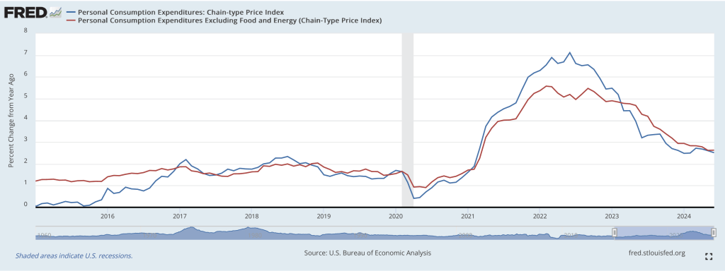
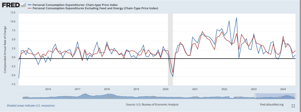
“We have stated that we do not expect it will be appropriate to reduce the target range for the federal funds rate until we have gained greater confidence that inflation is moving sustainably toward 2 percent. The second-quarter’s inflation readings have added to our confidence, and more good data would further strengthen that confidence. We will continue to make our decisions meeting by meeting.”

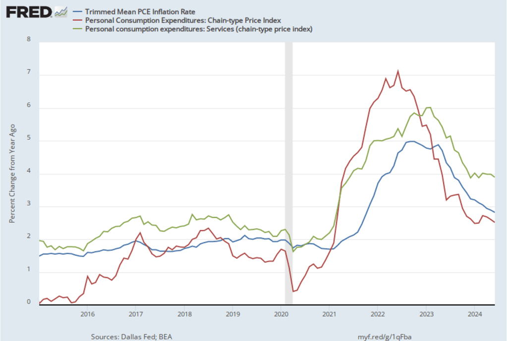
But in answering questions from reporters, he made it clear that—as many economists and Wall Street investors had already concluded—the FOMC was likely to reduce its target for the federal funds rate at its next meeting on September 17-18. Powell noted that recent data were consistent with the inflation rate continuing to decline toward the Fed’s 2 percent annual target. Powell summarized the consensus from the discussion among committee members as being that “the time was approaching for cutting rates.”

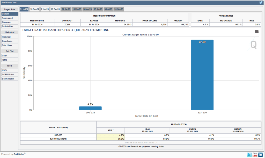
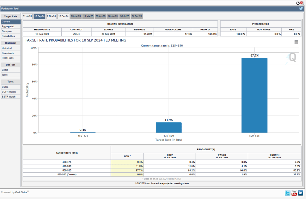
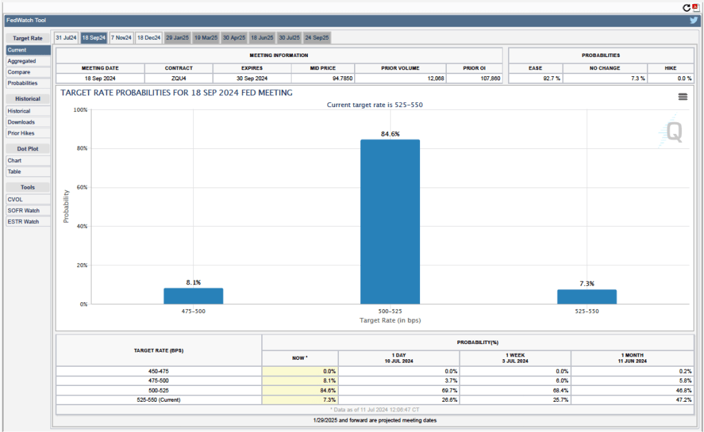
Futures markets allow investors to buy and sell futures contracts on commodities–such as wheat and oil–and on financial assets. Investors can use futures contracts both to hedge against risk—such as a sudden increase in oil prices or in interest rates—and to speculate by, in effect, betting on whether the price of a commodity or financial asset is likely to rise or fall. (We discuss the mechanics of futures markets in Chapter 7, Section 7.3 of Money, Banking, and the Financial System.) The CME Group was formed from several futures markets, including the Chicago Mercantile Exchange, and allows investors to trade federal funds futures contracts. The data that result from trading on the CME indicate what investors in financial markets expect future values of the federal funds rate to be. The following chart from the CME’s FedWatch Tool shows the current values resulting from trading of federal funds futures.

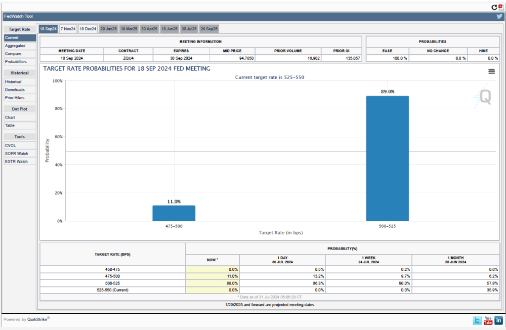
The probabilities in the chart reflect investors’ predictions of what the FOMC’s target for the federal funds rate will be after the committee’s September meeting. The chart indicates that investors assign a probability of 100 percent to the FOMC cutting its federal funds rate target at this meeting. Investors assign a probability of 89.0 percent that the committee will cut its target by 0.25 percentage point and a probability of 11.0 percent that the commitee will cut its target by 0.50 percentage point. When asked at his press conference whether the committee had given any consideration to making a 0.50 percentage point cut in its target, Powell said that it hadn’t.

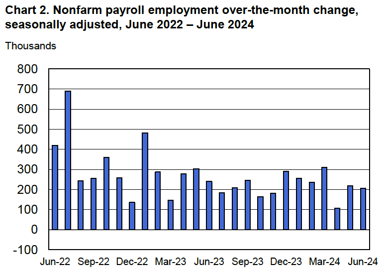
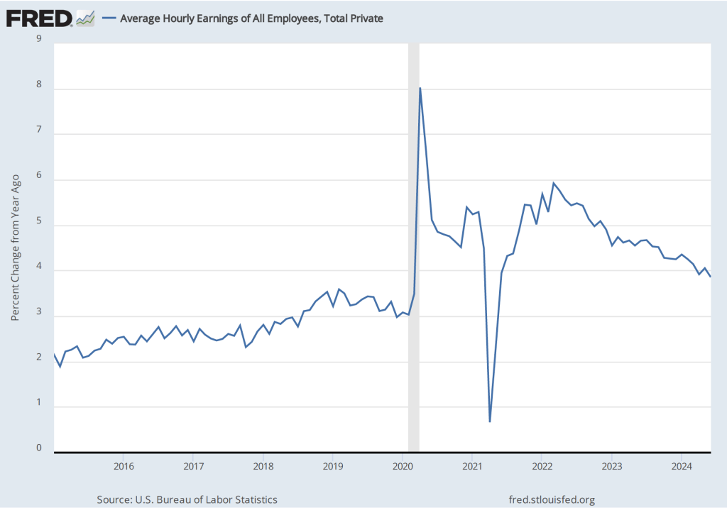
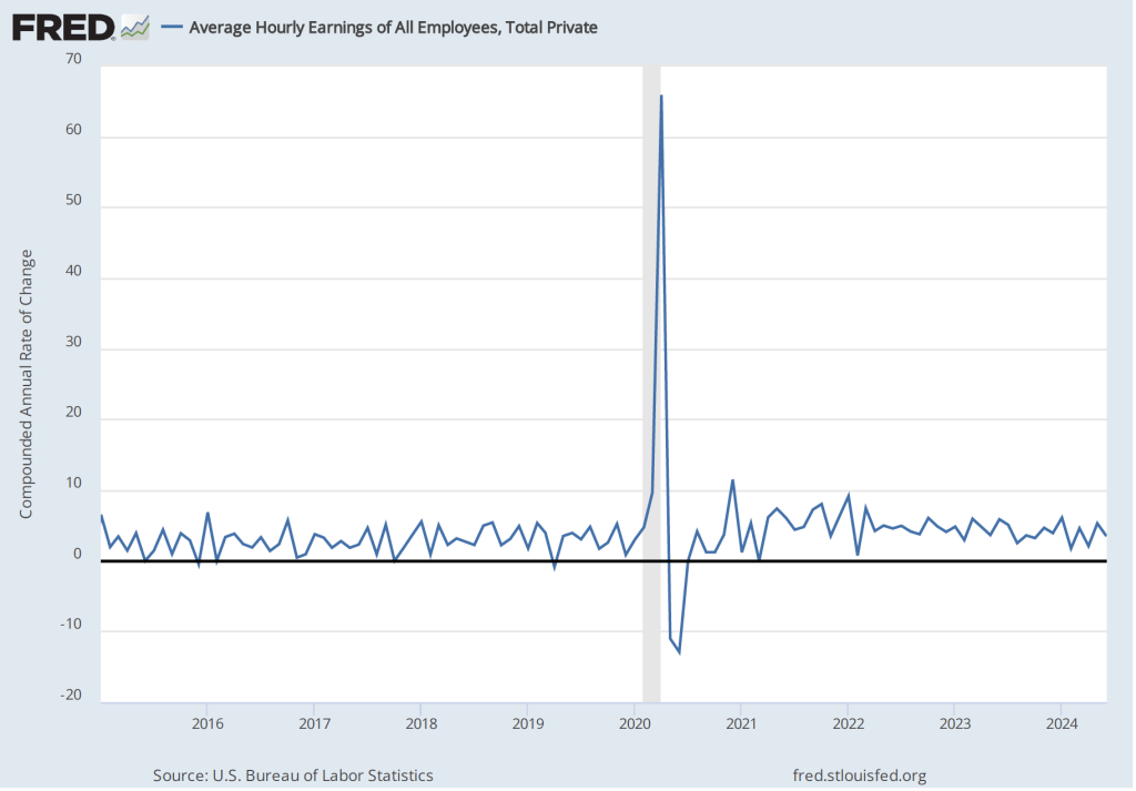
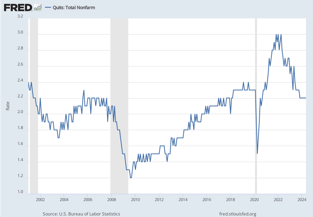
Powell stated that the latest data on wage increases had led the committee to conclude that the labor market was no longer a source of inflationary pressure. The morning of the press conference, the Bureau of Labor Statistics (BLS) released its latest report on the Employment Cost Index (ECI). As we’ve noted in earlier posts, as a measure of the rate of increase in labor costs, the FOMC prefers the ECI to average hourly earnings (AHE).

As a measure of how wages are increasing or decreasing during a particular period, AHE can suffer from composition effects because AHE data aren’t adjusted for changes in the mix of occupations workers are employed in. In contrast, the ECI holds the mix of occupations constant. The ECI does have the drawback that it is only available quarterly whereas the AHE is available monthly.

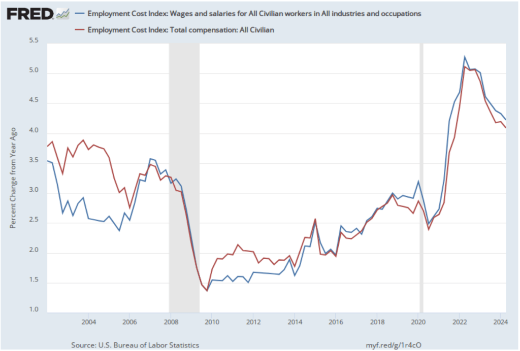
The following figure shows the percentage change in the ECI for all civilian workers from the same quarter in the previous year. The blue line looks only at wages and salaries, while the red line is for total compensation, including non-wage benefits like employer contributions to health insurance. The rate of increase in the wage and salary measure decreased slightly from 4.3 percent in the first quarter of 2024 to 4.2 percent in the second quarter of 2024. The rate of increase in compensation also declined slightly from 4.2 percent to 4.1 percent. As the figure shows, both measures continued their declines from the peak of wage inflation during the second quarter of 2022. In his press conference, Powell said that the this latest ECI report was a little better than the committee had expected.

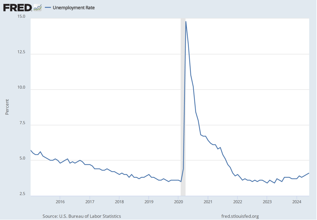
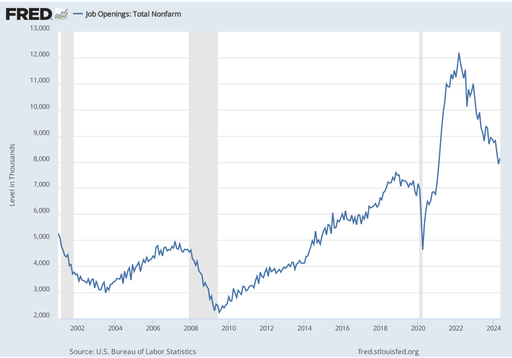
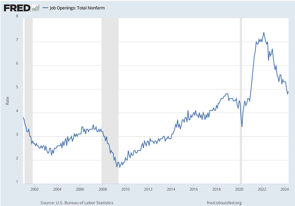
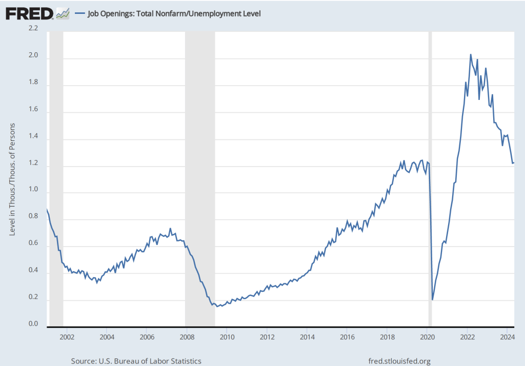
Finally, Powell noted that the committee saw no indication that the U.S. economy was heading for a recession. He observed that: “The labor market has come into better balance and the unemployment rate remains low.” In addition, he said that output continued to grow steadily. In particular, he pointed to growth in real final sales to private domestic purchasers. This macro variable equals the sum of personal consumption expenditures and gross private fixed investment. By excluding exports, government purchases, and changes in inventories, final sales to private domestic purchasers removes the more volatile components of gross domestic product and provides a better measure of the underlying trend in the growth of output.

As the following figure shows, this measure of output has grown at an annual rate of more than 2.5 percent in each of the last three quarters. Output expanding at that rate is indicative of an economy that is neither overheating nor heading toward a recession.

At this point, unless macro data releases are unexpectedly strong or weak during the next six weeks, it seems nearly certain that at its September meeting the FOMC will reduce its target range for the federal funds rate by 0.25 percentage point.

Latest PCE Report Shows Inflation Continues to Ease

Federal Reserve Chair Jerome Powell at a press conference following a meeting of the Federal Open Market Committee (Photo from federal reserve.gov)

Inflation in 2024 is a tale of two quarters. During the first quarter of 2024, inflation ran higher than expected considering the falling inflation rates at the end of 2023. As a result, although at the beginning of the year many economists and Wall Street analysts had expected the Federal Reserve’s policy-making Federal Open Market Committee (FOMC) would cut its target for the federal funds rate at least once in the first half of 2024, the FOMC left its target unchanged.

On July 26, the Bureau of Economic Analysis (BEA) released its “Personal Income and Outlays” report for June. The report includes monthly data on the personal consumption expenditures (PCE) price index. The Fed relies on annual changes in the PCE price index to evaluate whether it’s meeting its 2 percent annual inflation target. The report confirmed that PCE inflation slowed in the second quarter, bringing it closer to the Fed’s 2 percent target.

The following figure shows PCE inflation (blue line) and core PCE inflation (red line)—which excludes energy and food prices—for the period since January 2015 with inflation measured as the percentage change in the PCE from the same month in the previous year. Measured this way, in June PCE inflation (the blue line) was 2.5 percent, down slightly from PCE inflation of 2.6 percent in May. Core PCE inflation (the red line) in June was also 2.5 percent, which was unchanged from May.

The following figure shows PCE inflation and core PCE inflation calculated by compounding the current month’s rate over an entire year. (The figure above shows what is sometimes called 12-month inflation, while this figure shows 1-month inflation.) Measured this way, PCE inflation rose in June to 0.9 percent from 0.4 percent in May—although higher in June, inflation was well below the Fed’s 2 percent target in both months. Core PCE inflation rose from 1.5 percent in May to 2.0 percent in June. These data indicate that inflation has been at or below the Fed’s target for the last two months.

The following figure shows another way of gauging inflation by including the 12-month inflation rate in the PCE (the same as shown in the figure above—although note that PCE inflation is now the red line rather than the blue line), inflation as measured using only the prices of the services included in the PCE (the green line), and the trimmed mean rate of PCE inflation (the blue line). Fed Chair Jerome Powell and other members of the Federal Open Market Committee (FOMC) have said that they are concerned by the persistence of elevated rates of inflation in services. The trimmed mean measure is compiled by economists at the Federal Reserve Bank of Dallas by dropping from the PCE the goods and services that have the highest and lowest rates of inflation. It can be thought of as another way of looking at core inflation by excluding the prices of goods and services that had particularly high or particularly low rates of inflation during the month.

Inflation using the trimmed mean measure was 2.8 percent in June (calculated as a 12-month inflation rate), down only slightly from 2.9 percent in May—and still above the Fed’s target inflation rate of 2 percent. Inflation in services remained high in June at 3.9 percent, down only slightly from 4.0 percent in May.

This month’s PCE inflation data indicate that the inflation rate is still declining towards the Fed’s target, with the low 1-month inflation rates being particularly encouraging. It now seems likely that the FOMC will soon lower the committee’s target for the federal funds rate, which is currently 5.25 percent to 5.50 percent. Remarks by Fed Chair Powell have been interpreted as hinting as much. The next meeting of the FOMC is July 30-31. What do financial markets think the FOMC will decide at that meeting?

The probabilities in the chart reflect investors’ predictions of what the FOMC’s target for the federal funds rate will be after the committee’s July meeting. The chart indicates that investors assign a probability of only 4.7 percent to the FOMC cutting its federal funds rate target by 0.25 percentage point at its July 30-31 meeting and an 95.3 percent probability of the commitee leaving the target unchanged.

In contrast, the following figure shows that investors expect that the FOMC will cut its federal funds rate at the meeting scheduled for September 17-18. Investors assign an 87.7 percent probability of a 0.25 percentage point cut and a 11.9 percent probability of a 0.50 percentage point cut. The committee deciding to leave the target unchanged at 5.25 percent to 5.50 percent is effectively assigned a zero probability. In other words, investors believe with near certainty that the FOMC will reduce its target for the federal funds rate for the first time since the current round of rate increases ended in July 2023.

Every Day Is a Great Day For Economics. Let’s Solve Two (Exchange Rate) Problems.

Chicago Cubs Hall of Fame shortstop Ernie Banks was known for saying “It’s a great day for baseball. Let’s play two!” (Photo from the Baseball Hall of Fame)

First Solved Problem: Exchange Rates and Tourism

Supports: Macroeconomics, Chapter 18, Sections 18.2 and 18.6; and Economics, Chapter 28, Sections 28.2 and 28.6.

The headline of an article on nbcnews.com is: “The Fed May Soon Cut Interest Rates. That Could Make Your Next Trip Abroad More Expensive.”

Briefly explain the difference between a “strong dollar” and a “weak dollar.”
If you are going to spend two weeks on vacation in France, would you prefer that the dollar be strong or weak during that time? Briefly explain.
Briefly explain the connection between Federal Reserve monetary policy and the exchange rate between the U.S. dollar and other currencies.
Use your answers to parts a., b., and c. to explain what the headline means.

Solving the Problem

Step 1: Review the chapter material. This problem is about the effect of changes in exchange rates on import and export prices and the effect of changes in interest rates on exchange rates, so you may want to review Chapter 18, Sections 18.2 and 18.6.

Step 2: Answer part a. by explaining the difference between a “strong dollar” and a “weak dollar.” Generally, the U.S. dollar is called strong when it exchanges for more units of foreign currencies and is called weak when it exchanges for fewer units of foreign currencies. (Economists are less likely to use the phrases “strong dollar” and “weak dollar” than are members of the media.)

Step 3: Answer part b. by expalining whether you would like the U.S. dollar to be weak or strong during your vacation in France. France uses the euro as its currency. As a tourist, you will buy goods and services—such as restaurant meals and souvenirs—in euros. You would like the dollar to be strong because then you will be able to use fewer dollars to exhange for the euros you need to buy goods and services during your vacation.

Step 4: Answer part c. by explaining how Federal Reserve monetary policy affects the exchange rate. As we discuss in Section 18.6, when the Fed wants to pursue an expansionary monetary policy, the Federal Open Market Committee (FOMC) reduces its target for the federal funds rate, which typically results in other interest rates also declining. Lower interest rates make U.S. financial asses, such as Treasury bonds, less attractive relative to foreign financial assets, such as bonds issued by the French government. As a result the demand for U.S. dollars falls relative to the demand for foreign currencies, reducing the exchange rate between the dollar and other currencies. In other words, an expansionary monetary policy will result in a weaker dollar.

Step 5: Answer part d. by using your answers to parts a., b., and c. to expalin what the headline means. The headline indicates that the Fed may soon engage in an expansionary monetary policy, which will result in lower interest rates in the United States, leading to a weaker U.S. dollar. The weaker the dollar, the more dollars you will have to exchange to receive the same number of units of a foreign currency, causing you to have to spend more dollars to pay for the same goods and services during your trip. So, the Fed taking action to reduce interest rates will make your trip abroad more expensive.

Second Solved Problem: Solved Problem: Javier Milei and Argentina’s Exchange Rate Policy

Supports: Macroeconomics, Chapter 18, Sections 18.2 and 18.3; and Economics, Chapter 28, Sections 28.2 and 28.3.

Javier Milei was elected president of Argentina in December 2023. During the presidential campaign he proposed using market-based policies to address Argentina’s economic problems, particularly high rates of inflation and low rates of economic growth. One part of his program involves moving the government away from controlling the value of the peso either by allowing it to float or by making the U.S. dollar legal tender in Argentina. Initially, however, although Milei devalued the peso against the dollar, he didn’t allow the peso to float, keeping the peso pegged against the value of the dollar. An article in the Economist states that many economists believe that the peso is overvalued. The article notes that: “A pricey peso scares off tourists, makes exports expensive and deters investors.” The article also notes that allowing the peso to float “would probably push up inflation.”

Briefly explain what it means for a government to allow its currency to float.
What does it mean to say that a county’s currency is overvalued?
What does the article mean by a “pricey peso”? Why would a pricey peso scare off tourists, make exports expensive, and deter investors?
Why would allowing the peso to float probably push up inflation?

Solving the Problem

Step 1: Review the chapter material. This problem is about exchange rates and exchange rate systems, so you may want to review Chapter 18, Sections 18.2 18.3.

Step 2: Answer part a. by explaining what it means for a government to allow its currency to float. As we discuss in Section 18.3, when a government allows its currency to float it allows the exchange rate between its currency and other currencies to be determined by demand and supply in foreign exchange markets.

Step 3: Answer part b. by expalining what it means for a country’s currency to be overvalued. A currency is overvalued if a government pegs the exchange rate above the market equilibrium exchange rate.

Step 4: Answer part c. by explaining what a “pricey peso” means and why a pricey peso might scare off tourists, make exports expensive, and deter investors. In the context of this article, a pricey peso means an overvalued peso—one that is pegged above the market equilibrium exchange rate, as we noted in the answer to part b. If the peso is overvalued relative to other currencies, then tourists from those countries will find the prices of goods and services in Argentina to be high relative to the prices of those goods and services priced in their domestic currencies. We would expect that fewer foreing tourists would visit Argentina. A pricey peso would make the prices of Argentine exports higher in terms of U.S. dollars, euros, and other currencies. Those high prices will cause a decline in Argentine exports. Finally, a pricey peso will also discourage foreign investors from investing in Argentina because they will receive fewer units of their domestic currency in exchange for the pesos they earn from their investments in Argentina.

Step 5: Answer part d. by explaining why the Argentine government allowing the peso to float would likely increase inflation. The Argentine peso is overvalued, so allowing it to float will cause the value of the peso to decline relative to other currencies. As a result, the peso price of imports will increase. The prices of imported goods and services are included in the price indexes used to measure inflation, so floating the peso will likely increase the inflation rate in Argentina.

How Should the Fed Interpret the Monthly Employment Reports?

Jerome Powell arriving to testify before Congress. (Photo from Bloomberg News via the Wall Street Journal.)

Each month the Bureau of Labor Statistics (BLS) releases its “Employment Situation” report. As we’ve discussed in previous blog posts, discussions of the report in the media, on Wall Street, and among policymakers center on the estimate of the net increase in employment that the BLS calculates from the establishment survey.

How should the members of the Fed’s policy-making Federal Open Market Committee interpret these data? For instance, the BLS reported that the net increases in employment in June was 206,000. (Always worth bearing in mind that the monthly data are subject to—sometimes substantial—revisions.) Does a net increase of employment of that size indicate that the labor market is still running hot—with the quantity of labor demanded by businesses being greater than the quantity of labor workers are supplying—or that the market is becoming balanced with the quantity of labor demanded roughly equal to the quantity of labor supplied?

On July 9, in testimony before the Senate Banking Committee indicated that his interpretation of labor market data indicate that: “The labor market appears to be fully back in balance.” One interpretation of the labor market being in balance is that the number of net new jobs the economy creates is enough to keep up with population growth. In recent years, that number has been estimated to be 70,000 to 100,000. The number is difficult to estimate with precision for two main reasons:

There is some uncertainty about the number of older workers who will retire. The more workers who retire, the fewer net new jobs the economy needs to create to accommodate population growth.
More importantly, estimates of population growth are uncertain, largely because of disagreements among economists and demographers over the number of immigrants who have entered the United States in recent years.

In calculating the unemployment rate and the size of the labor force, the BLS relies on estimates of population from the Census Bureau. In a January report, the Congressional Budget Office (CBO) argued that the Census Bureau’s estimate of the population of the United States is too low by about 6 million people. As the following figure from the CBO report indicates, the CBO believes that the Census Bureau has underestimated how much immigration has occurred and what the level of immigration is likely to be over the next few years. (In the figure, SSA refers to the Social Security Administration, which also makes forecasts of population growth.)

Some economists and policymakers have been surprised that low levels of unemployment and large monthly increases in employment have not resulted in greater upward pressure on wages. If the CBO’s estimates are correct, the supply of labor has been increasing more rapidly than is indicated by census data, which may account for the relative lack of upward pressure on wages. If the CBO’s estimates of population growth are correct, a net increase in employment of 200,000, as occured in June, may be about the number necessary to accommodate growth in the labor force. In other words, Chair Powell would be correct that the labor market was in balance in June.

In a recent publication, economists Nicolas Petrosky-Nadeau and Stephanie A. Stewart of the Federal Reserve Bank of San Francisco look at a related concept: breakeven employment growth—the rate of employment growth required to keep the unemployment rate unchanged. They estimate that high rates of immigration during the past few years have raised the rate of breakeven employment growth from 70,000 to 90,000 jobs per month to 230,000 jobs per month. This analysis would be consistent with the fact that as net employment increases have averaged 177,000 over the past three months—somewhat below their estimate of breakeven employment growth—the unemployment rate has increased from 3.8 percent to 4.1 percent.

Latest CPI Report Shows Inflation Continuing to Slow

Image of “a family shopping in a supermarket” generated by ChatGTP 4o.

In testifying before Congress this week, Federal Reserve Chair Jerome Powell indicated that the Fed’s policy-making Federal Open Market Committee (FOMC) was becoming more concerned that it not be too late in reducing its target for the federal funds rate:

“[I]n light of the progress made both in lowering inflation and in cooling the labor market over the past two years, elevated inflation is not the only risk we face. Reducing policy restraint too late or too little could unduly weaken economic activity and employment.”

Powell also noted that: “more good data would strengthen our confidence that inflation is moving sustainably toward 2 percent.” Today (July 11), Powell received more good data as the Bureau of Labor Statistics (BLS) released its monthly report on the consumer price index (CPI), which showed a further slowing in inflation.

As the following figure shows, the inflation rate for June measured by the percentage change in the CPI from the same month in the previous month—headline inflation (the blue line)—was 3.o percent down from 3.3 percent in May. Core inflation (the red line)—which excludes the prices of food and energy—was 3.3 percent in June, down from 3.4 percent in May.

As the following figure shows, if we look at the 1-month inflation rate for headline and core inflation—that is the annual inflation rate calculated by compounding the current month’s rate over an entire year—the declines in the inflation rate are much larger. Headline inflation (the blue line) declined from 0.1 percent in May to –0.7 in June—consumer prices fell during June. Core inflation (the red line) declined from 2.0 percent in May to 0.8 percent in June. Overall, we can say that inflation has cooled further in June, bringing the U.S. economy closer to a soft landing—with the annual inflation rate returning to the Fed’s 2 percent target without the economy being pushed into a recession. (Note, though, that the Fed uses the personal consumption expenditures (PCE) price index, rather than the CPI in evaluating whether it is hitting its 2 percent inflation target.)

The FOMC has been looking closely at inflation in the price of shelter. The price of “shelter” in the CPI, as explained here, includes both rent paid for an apartment or house and “owners’ equivalent rent of residences (OER),” which is an estimate of what a house (or apartment) would rent for if the owner were renting it out. OER is included to account for the value of the services an owner receives from living in an apartment or house.

As the following figure shows, inflation in the price of shelter has been a significant contributor to headline inflation. The blue line shows 12-month inflation in shelter and the red line shows 1-month inflation in shelter. Twelve-month inflation in shelter continued its decline that began in the spring of 2023. One-month inflation in shelter declined substantially from 4.9 percent in May to 2.1 percent in June. These values indicate that the price of shelter may no longer be a significant driver of headline inflation.

Finally, in order to get a better estimate of the underlying trend in inflation, some economists look at median inflation and trimmed mean inflation. Meadin inflation is calculated by economists at the Federal Reserve Bank of Cleveland and Ohio State University. If we listed the inflation rate in each individual good or service in the CPI, median inflation is the inflation rate of the good or service that is in the middle of the list—that is, the inflation rate in the price of the good or service that has an equal number of higher and lower inflation rates. Trimmed mean inflation drops the 8 percent of good and services with the higherst inflation rates and the 8 percent of goods and services with the lowest inflation rates.

As the following figure (from the Federal Reserve Bank of Cleveland) shows, both median inflation (the brown line) and trimmed mean inflation (the blue line) were somewhat higher than either headline CPI inflation or core CPI inflation. One conclusion from these data is that headline and core inflation may be somewhat understating the underlying rate of inflation.

Financial markets are interpreting the most inflation and employment data as indicating that at its meeting on Septembe 17-18 the FOMC is likely to cut its target range for the federal funds rate from the current 5.25 percent to 5.50 to 5.00 percent to 5.25 percent.

The probabilities in the chart reflect investors’ predictions of what the FOMC’s target for the federal funds rate will be after the committee’s September meeting. The chart indicates that investors assign a probability of only 8.1 percent to the FOMC leaving its federal funds rate target unchanged at its September meeting, but a 84.6 percent probability of the committee cutting its target by 0.25 percentage point (and a 7.3 percent probability of the committee cutting its target by 0.50 percent age point).

Latest Jobs Report May Indicate the Labor Market Is Weakening

Image generated by ChatGTP 4o.

Recent macroeconomic data have been sending mixed signals about the state of the U.S. economy. The growth in real GDP, industrial production, retail sales, and real consumption spending has been slowing. Growth in employment has been a bright spot—showing steady net increases in job growth above the level necessary to keep up with population growth. Even here, though, as we discuss in a recent blog post, the data may be overstating the actual strength of the labor market.

This morning (July 5), the Bureau of Labor Statistics (BLS) released its “Employment Situation” report (often referred to as the “jobs report”) for June, which, while seemingly indicating continued strong job growth, also provides some indications that the labor market may be weakening. The jobs report has two estimates of the change in employment during the month: one estimate from the establishment survey, often referred to as the payroll survey, and one from the household survey. As we discuss in Macroeconomics, Chapter 9, Section 9.1 (Economics, Chapter 19, Section 19.1), many economists and policymakers at the Federal Reserve believe that employment data from the establishment survey provides a more accurate indicator of the state of the labor market than do either the employment data or the unemployment data from the household survey. (The groups included in the employment estimates from the two surveys are somewhat different, as we discuss in this post.)

According to the establishment survey, there was a net increase of 206,000 jobs during April. This increase was a little above the increase of 1900,000 to 200,000 that economists had forecast in surveys by the Wall Street Journal and bloomberg.com. The following figure, taken from the BLS report, shows the monthly net changes in employment for each month during the past to years.

It’s notable that the previously reported increases in employment for April and May were revised downward by 110,000 jobs, or by about 25 percent. (The BLS notes that: “Monthly revisions result from additional reports received from businesses and government agencies since the last published estimates and from the recalculation of seasonal factors.”) As we’ve discussed in previous posts (most recently here), revisions to the payroll employment estimates can be particularly large at the beginning of a recession.

As the following figure shows, the net change in jobs from the household survey moves much more erratically than does the net change in jobs in the establishment survey. The net increase in jobs as measured by the household survey increased from –408,000 in May (that is, employment by this measure fell during May) to 116,000 in June.

Note that the BLS also reports a survey for household employment adjusted to conform to the concepts and definitions used to construct the payroll employment series. After this adjustment, over the past 12 months household employment has increased by 32.5 million less than has payroll employment. Clearly, this is a very large discrepancy and may be indicating that the payroll survey is substantially overstating growth in employment.

The unemployment rate, which is also reported in the household survey, ticked up slightly from 4.0 percent to 4.1 percent. Although still low by historical standards, June was the fourth consecutive month in which the unemployment rate increased.

The establishment survey also includes data on average hourly earnings (AHE). As we note in this post, many economists and policymakers believe the employment cost index (ECI) is a better measure of wage pressures in the economy than is the AHE. The AHE does have the important advantage that it is available monthly, whereas the ECI is only available quarterly. The following figure show the percentage change in the AHE from the same month in the previous year. The 3.9 percent increase for June continues a downward trend that began in January and is the smallest increase since June 2021.

The following figure shows wage inflation calculated by compounding the current month’s rate over an entire year. (The figure above shows what is sometimes called 12-month wage inflation, whereas this figure shows 1-month wage inflation.) One-month wage inflation is much more volatile than 12-month inflation—note the very large swings in 1-month wage inflation in April and May 2020 during the business closures caused by the Covid pandemic.

The 1-month rate of wage inflation of 3.5 percent in June is a significant decrease from the 5.3 percent rate in May, although it’s unclear whether the decline was an additional sign that the labor market is weakening or reflected the greater volatility in wage inflation when calculated this way.

What effect is today’s job reports likely to have on the Fed’s policy-making Federal Open Market Committee as it considers changes in its target for the federal funds rate? As always, it’s a good idea not to rely too heavily on a single data point—particularly because, as we noted earlier, the establishment survey employment data is subject to substantial revisions. But the Wall Street Journal’s headline that the “Case for September Rate Cut Builds After Slower Jobs Data,” seems likely to be accurate.

Latest JOLTS Report Confirms that the Labor Market Is Returning to Pre-Pandemic Conditions

When inflation began to accelerate in the spring of 2022, the highly unusual situation in the U.S. labor market was one of the reasons. This morning (July 2), the Bureau of Labor Statistics (BLS) released its “Job Openings and Labor Turnover” (JOLTS) report for May 2024. The report proivided more data indicating that the U.S. labor market is continuing its return to pre-pandemic conditions.

The following figures shows the total number of job openings. The BLS defines a job opening as a full-time or part-time job that a firm is advertising and that will start within 30 days. Although the total number of job openings, at 8.1 million, is still somewhat above pre-pandemic levels, it has been gradually declining since reaching a peak of 12.2 million in March 2022.

The next figure shows that, at 4.9 percent, the rate of job openings has continued its slow decline from 7.4 percent in March 2022. The rate in May was just slightly above the rate in January 2019, although it was till above the rates during most of 2019 and early 2020, as well as the rates during most of the period following the Great Recession of 2007–2009. The rate of job openings is defined by the BLS as the number of job openings divided by the number of job openings plus the number of employed workers, multiplied by 100.

In the following figure, we compare the total number of job openings to the total number of people unemployed. The figure shows a slow decline from a peak of more than 2 job openings per unemployed person in the spring of 2022 to 1.2 job openings per employed person in May 2024—the same as in April and about the same as in 2019 and early 2020, before the pandemic. Note that the number is still above 1.0, indicating that the demand for labor is still high, although no higher than during the strong labor market of 2019.

The rate at which workers are willing to quit their jobs is an indication of how they perceive the ease of finding a new job. As the following figure shows, the quit rate declined slowly from a peak of 3 percent in late 2021 and early 2022 to 2.2 percent in November 2023, where it has remained through May 2024. That rate is slightly below the rate during 2019 and early 2020. By this measure, workers perceptions of the state of the labor market seem largely unchanged in recent months.

The JOLTS data indicate that the labor market is about as strong as it was in the months priod to the start of the pandemic, but it’s not as historically tight as it was through most of 2022 and 2023. Speaking today at a conference hosted by the European Central Bank, Fed Chair Jerome Powell was quoted as saying that the Fed had made “a lot of progress” in reducing inflation and that the labor market had made “a pretty substantial” move toward a better balance between labor demand and labor supply.

On Friday morning, the BLS will release its “Employment Situation” report for June, which will provide additional data on the state of the labor market. (Note that the data in the JOLTS report lag the data in the “Employment Situation” report by one month.)

Latest PCE Report Shows Inflation Slowing

Chair Jerome Powell and other members of the Federal Open Market Committee (Photo from federalreserve.gov)

On Friday, June 28, the Bureau of Economic Analysis (BEA) released its “Personal Income and Outlays” report for April, which includes monthly data on the personal consumption expenditures (PCE) price index. Inflation as measured by annual changes in the consumer price index (CPI) receives the most attention in the media, but the Federal Reserve looks instead to inflation as measured by annual changes in the PCE price index to evaluate whether it’s meeting its 2 percent annual inflation target.

The following figure shows PCE inflation (blue line) and core PCE inflation (red line)—which excludes energy and food prices—for the period since January 2015 with inflation measured as the change in the PCE from the same month in the previous year. Measured this way, in May PCE inflation (the blue line) was 2.6 percent in May, down slightly from PCE inflation of 2.7 percent in April. Core PCE inflation (the red line) in May was also 2.6 percent, down from 2.8 percent in April.

The following figure shows PCE inflation and core PCE inflation calculated by compounding the current month’s rate over an entire year. (The figure above shows what is sometimes called 12-month inflation, while this figure shows 1-month inflation.) Measured this way, PCE inflation sharply declined from 3.2 percent in April to -0.1 percent in in May—meaning that consumer prices actually fell during May. Core PCE inflation declined from 3.2 percent in April to 1.0 percent in May. This decline indicates that inflation by either meansure slowed substantially in May, but data for a single month should be interpreted with caution.

Inflation using the trimmed mean measure was 2.8 percent in May (calculated as a 12-month inflation rate), down only slightly from 2.9 percent in April—and still well above the Fed’s target inflation rate of 2 percent. Inflation in services remained high in May at 3.9 percent, down only slightly from 4.0 percent in April.

This month’s PCE inflation data indicate that the inflation rate is still declining towards the Fed’s target, with the low 1-month inflation rates being particularly encouraging. But the FOMC will likely need additional data before deciding to lower the committee’s target for the federal funds rate, which is currently 5.25 percent to 5.50 percent. The next meeting of the FOMC is July 30-31. What do financial markets think the FOMC will decide at that meeting?

The probabilities in the chart reflect investors’ predictions of what the FOMC’s target for the federal funds rate will be after the committee’s July meeting. The chart indicates that investors assign a probability of only 10.3 percent to the FOMC cutting its federal funds rate target by 0.25 percentage point at that meeting and an 89.7 percent probability of the commitee leaving the target unchanged.

In contrast, the following figure shows that investors expect that the FOMC will cut its federal funds rate at the meeting scheduled for September 17-18. Investors assign a 57.9 percent probability of a 0.25 percentage point cut and a 6.2 percent probability of a 0.50 percentage point cut. The committee deciding to leave the target unchanged at 5.25 percent to 5.50 percent is assigned a probability of only 35.9 percent.

Is the U.S Labor Market Weaker Than It Seems?

The monthly “Employment Situation” report from the Bureau of Labor Statistics (BLS) is closely watched by economists, investment analysts, and Federal Reserve policymakers. Many economists believe that the payroll employment data from the report is the best single indicator of the current state of the economy.

Most economists, inside and outside of the government, accept the dates determined by the Business Cycle Dating Committee of the National Bureau of Economic Research (NBER) for when a recession begins and ends. Although that committee takes into account a variety of macroeconomic data series, the peak of a business cycle as determined by the committee almost always corresponds to the peak in payroll employment and the trough of a business cycle almost always corresponds to the trough in payroll employment.

One drawback to relying too heavily on payroll employment data in gauging the state of the economy is that the data are subject to—sometimes substantial—revisions. As the BLS explains: “Monthly revisions result from additional reports received from businesses and government agencies since the last published estimates and from the recalculation of seasonal factors.” The revisions can be particularly large at the beginning of a recession.

For example, the following figure shows revisions the BLS made to its initial estimates of the change in payroll employment during the months around the 2007–2009 recession. The green bars show months for which the BLS revised its preliminary estimates to show that fewer jobs were lost (or that more jobs were created), and the red bars show months for which the BLS revised its preliminary estimates to show that more jobs were lost (or that fewer jobs were created).

For example, the BLS initially reported that employment declined by 159,000 jobs during September 2008. In fact, after additional data became available, the BLS revised its estimate to show that employment had declined by 460,000 jobs during the month—a difference of 300,000 more jobs lost. As the recession deepened between April 2008 and April 2009, the BLS’s initial reports underestimated the number of jobs lost by 2.3 million. In other words, the recession of 2007–2009 turned out to be much more severe than economists and policymakers realized at the time.

The BLS also made substantial revisions to its initial estimates of payroll employment for 2020 and 2021 during the Covid pandemic, as the following figure shows. (Note that this figure appears in our new 9th edition of Macroeconomics, Chapter 9, Section 9.1 (Economics, Chapter 19, Section 19.1 and Essentials of Economics, Chapter 13, Section 13.1).)

The BLS initially estimated that employment in March 2020 declined by about 700,000. After gathering more data, the BLS revised its estimate to indicate that employment declined by twice as much. Similarly, the BLS’s initial estimates substantially understated the actual growth in employment from August to December 2021. After gathering more data, the BLS revised its estimate to indicate that nearly 2 million more jobs had been created during those months than it had originally estimated.

Just as the initial estimates for total payroll employment are often revised by sutbstantial amounts up or down, the same is true of the initial estimates of payroll employment in individual industries. Because the number of establishments surveyed in any particular industry can be small, the initial estimates can be highly inaccurate. For instance, Justin Fox, a columnist for bloomberg.com recently noted what appears to be a surge in employment in the “sports teams and clubs” industry. As the following figure shows, employment in this industry seems to have increased by an improbably large 75 percent. Was there a sudden increase in the United States in the number of new sports teams? Certainly not over just a few months. It’s more likely that most of the increase in employment in this industry will disappear when the initial employment estimates are revised.

One source of data for the BLS revisions to the monthly payroll employment data is the BLS’s “Quarterly Census of Employment and Wages.” The QCEW is based on the reports required of all firms that participate in the state and federal unemployment insurance program. The BLS estimates that 95 percent of all jobs in the United States are included in the QCEW data. As a result, the QCEW surveys about 11.9 million establishments as opposed to the 666,000 establishments included in the establishment survey.

The BLS uses the QCEW to benchmark the payroll employment data, which reconciles the two series. The BLS makes the revisions with a lag. For instance, the payroll employment data for 2023 won’t be revised using the QCEW data until August 2024. Looking at the 2023 employment data from the two series shows a large discrepancy, as seen in the following figure.

The blue line shows the employment data from the establishment survey and the orange line shows the data from the QCEW survey. (Both series are of nonseasonally adjusted data.) The values on the vertical axis are thousands of workers. In December 2023, the establishment survey indicated that a total of 158,347,000 people were employed in the nonfarm sector in the United States. The QCEW series shows a total of 154,956,133 people were employed in the nonfarm sector—about 3.4 million fewer.

How can we interpret the discrepancy between the employment totals from the two series? The most straightforward interpretation is that the QCEW data, which uses a larger sample, is more accurate and payroll employment has been significantly overstating the level of employment in the U.S. economy. In other words, the labor market was weaker in 2023 than it seemed, which may help to explain why inflation slowed as much as it did, particularly in the second half of the year.

However, this interpretation is not clear cut because the QCEW data are also subject to revision. As Ernie Tedeschi, director of economics at the Budget Lab at Yale and former chief economist for the Council of Economic Advisers, has pointed out, the QCEW data are typically revised upwards, which would close some of the gap between the two series. So, although it seems likely that the closely watched payroll employment data have overstated the strength of the labor market, we won’t get a clearer indication of how large the overstatement is until August when the BLS will use the QCEW data to benchmark the payroll employment data.

Latest CPI Report Shows Slowing Inflation and the FOMC Appears Likely to Cut Its Target for the Federal Funds Rate at Least Once This Year

Image of “a woman shopping in a grocery store” generated by ChatGTP 4o.

Today (June 12) we had the unusual coincidence of the Bureau of Labor Statistics (BLS) releasing its monthly report on the consumer price index (CPI) on the same day that the Federal Open Market Committee (FOMC) concluded a meeting. The CPI report showed that the inflation rate had slowed more than expected. As the following figure shows, the inflation rate for May measured by the percentage change in the CPI from the same month in the previous month—headline inflation (the blue line)—was 3.3 percent—slightly below the 3.4 percent rate that economists surveyed by the Wall Street Journal had expected, and slightly lower than the 3.4 percent rate in April. Core inflation (the red line(—which excludes the prices of food and energy—was 3.4 percent in May, down from 3.6 percent in April and slightly lower than the 3.5 percent rate that economists had been expecting.

As the following figure shows, if we look at the 1-month inflation rate for headline and core inflation—that is the annual inflation rate calculated by compounding the current month’s rate over an entire year—the declines in the inflation rate are much larger. Headline inflation (the blue line) declined from 3.8 percent in April to 0.1 percent in May. Core inflation (the red line) declined from 3.6 percent in April to 2.0 percent in May. Overall, we can say that inflation has cooled in May and if inflation were to continue at the 1-month rate, the Fed will have succeeded in bringing the U.S. economy in for a soft landing—with the annual inflation rate returning to the Fed’s 2 percent target without the economy being pushed into a recession.

But two important notes of caution:

1. It’s hazardous to rely to heavily on data from a single month. Over the past year, the BLS has reported monthly inflation rates that were higher than economists expected and rates that was lower than economists expected. The current low inflation rate would have to persist over at least a few more months before we can safely conclude that the Fed has achieved a safe landing.

2. As we discuss in Macroeconomics, Chapter 15, Section 15.5 (Economics, Chapter 25, Section 25.5), the Fed uses the personal consumption expenditures (PCE) price index, rather than the CPI in evaluating whether it is hitting its 2 percent inflation target. So, today’s encouraging CPI data would have to carry over to the PCE data that the Bureau of Economic Analysis (BEA) will release on January 28 before we can conclude that inflation as the Fed tracks it did in fact slow significantly in April.

The BLS released the CPI report at 8:30 am eastern time. The FOMC began its meeting later in the day and so committee members were able to include in their deliberations today’s CPI data along with other previously available information on the state of the economy. At the close of the meeting, , the FOMC released a statement in which it stated, as expected, that it would leave its target range for the federal funds rate unchanged at 5.25 percent to 5.50 percent. After the meeting, the committee also released—as it typically does at its March, June, September, and December meetings—a “Summary of Economic Projections” (SEP), which presents median values of the committee members’ forecasts of key economic variables. The values are summarized in the following table, reproduced from the release.

The table shows that compared with their projections in March—the last time the FOMC published the SEP—committee members were expecting higher headline and core PCE inflation and a higher federal funds rate at the end of this year. In the long run, committee members were expecting a somewhat highr unemployment rate and somewhat higher federal funds rate than they had expected in March.

Note, as we discuss in Macreconomics, Chapter 14, Section 14.4 (Economics, Chapter 24, Section 24.4 and Essentials of Economics, Chapter 16, Section 16.4), there are twelve voting members of the FOMC: the seven members of the Board of Governors, the president of the Federal Reserve Bank of New York, and presidents of four of the other 11 Federal Reserve Banks, who serve one-year rotating terms. In 2024, the presidents of the Richmond, Atlanta, San Francisco, and Cleveland Feds are voting members. The other Federal Reserve Bank presidents serve as non-voting members, who participate in committee discussions and whose economic projections are included in the SEP.

Prior to the meeting there was much discussion in the business press and among investment analysts about the dot plot, shown below. Each dot in the plot represents the projection of an individual committee member. (The committee doesn’t disclose which member is associated with which dot.) Note that there are 19 dots, representing the 7 members of the Fed’s Board of Governors and all 12 presidents of the Fed’s district banks.

The plots on the far left of the figure represent the projections of each of the 19 members of the value of the federal funds rate at the end of 2024. Four members expect that the target for the federal funds rate will be unchanged at the end of the year. Seven members expect that the committee will cut the target range once, by 0.25 percentage point, by the end of the year. And eight members expect that the cut target range twice, by a total of 0.50 percent point, by the end of the year. Members of the business media and financial analysts were expecting tht the dot plot would project either one or two target rate cuts by the end of the year. The committee was closely divided among those two projections, with the median projection being for a single rate cut.

In its statement following the meeting, the committee noted that:

“In considering any adjustments to the target range for the federal funds rate, the Committee will carefully assess incoming data, the evolving outlook, and the balance of risks. The Committee does not expect it will be appropriate to reduce the target range until it has gained greater confidence that inflation is moving sustainably toward 2 percent. In addition, the Committee will continue reducing its holdings of Treasury securities and agency debt and agency mortgage‐backed securities. The Committee is strongly committed to returning inflation to its 2 percent objective.”

In his press conference after the meeting, Fed Chair Jerome Powell noted that the morning’s CPI report was a “Better inflation report than nearly anyone expected.” But, Powell also noted that: “You don’t want to be motivated any one data point.” Reinforcing the view quoted above in the committee’s statement, Powell emphasized that before cutting the target for the federal funds rate, the committee would need “Greater confidence that inflation is moving back to 2% on a sustainable basis.”

In summary, today’s CPI report was an indication that the Fed is on track to bring about a soft landing, but the FOMC will be closely analyzing macroeconomic data over at least the next few months before it is willing to cut its target for the federal funds rate.