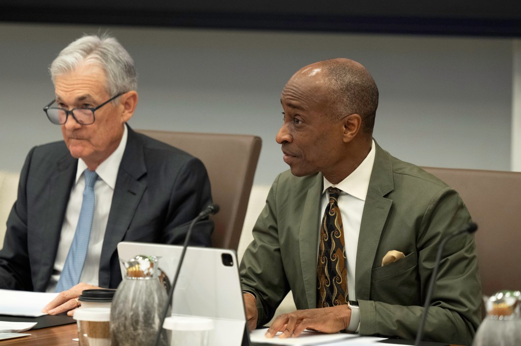
Photo of Fed Chair Jerome Powell from federalreserve.gov
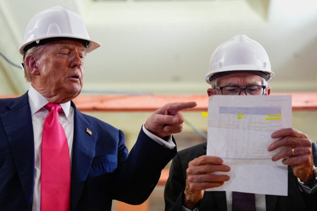
Today’s meeting of the Federal Reserve’s policymaking Federal Open Market Committee (FOMC) occurred against a backdrop of President Trump pressuring the committee to reduce its target for the federal funds rate. In a controversial move, Trump nominated Stephen Miran, chair of Council of Economic Advisers (CEA), to fill an open seat on the Fed’s Board of Governors. Miran took a leave of absence from the CEA rather than resign his position, which made him the first member of the Board of Governors in decades to maintain an appointment elsewhere in the executive branch while serving on the Board. In addition, Trump had fired Governor Lisa Cook on the grounds that she had committed fraud in applying for a mortgage at a time before her appointment to the Board. Cook denied the charge and a federal appeals court sustained an injunction allowing her to participate in today’s meeting.
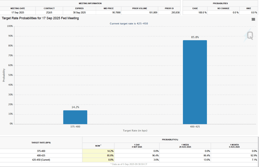
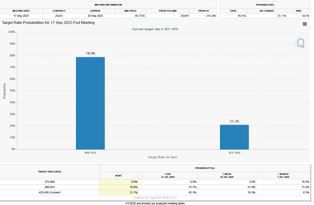
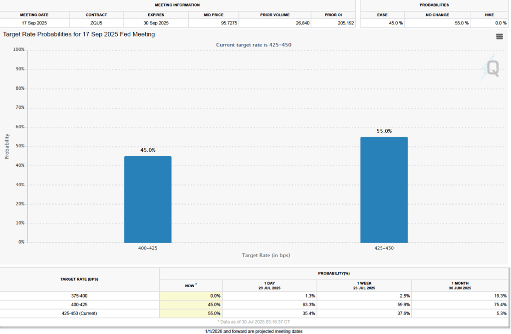
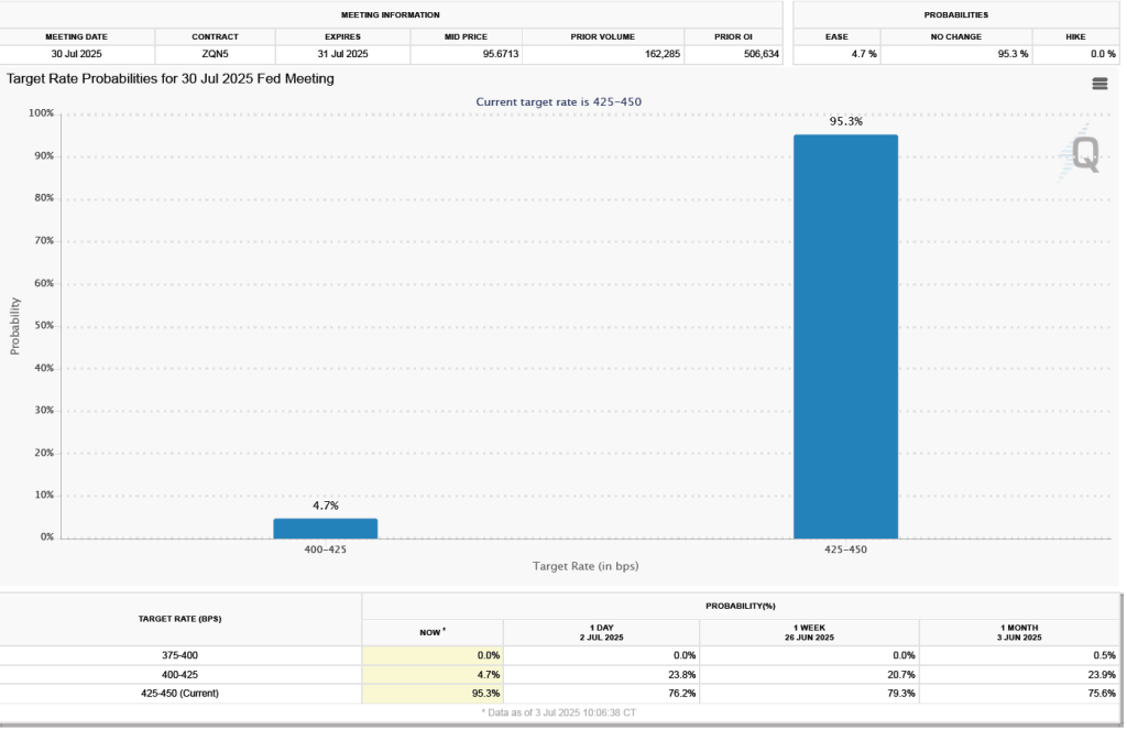
As most observers had expected, the committee decided today to lower its target for the federal funds rate from a range of 4.25 percent to 4.50 percent to a range of 4.00 percent to 4.25 percent—a cut of 0.25 percentage point, or 25 basis points. The members of the committee voted 11 to 1 for the 25 basis point cut with Miran dissenting because he preferred a 50 basis point cut.
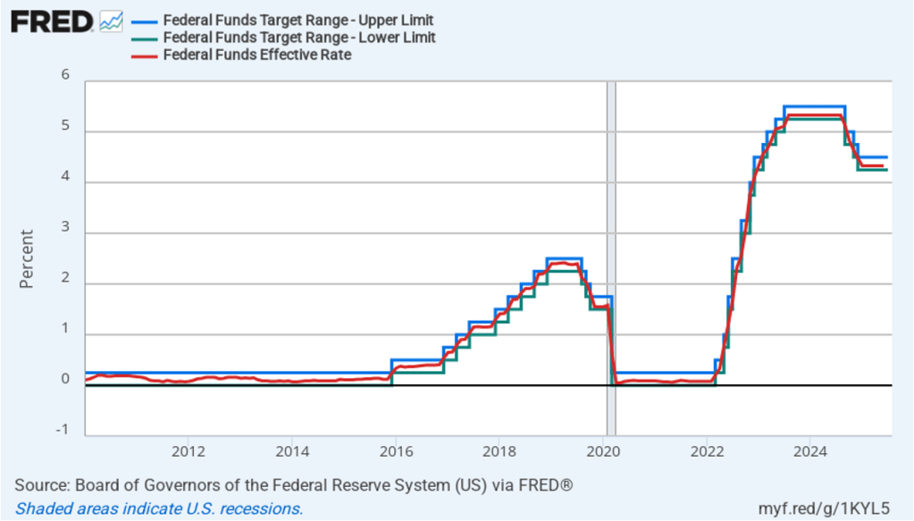
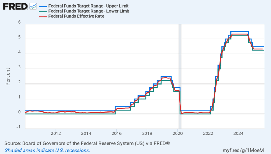
The following figure shows, for the period since January 2010, the upper bound (the blue line) and lower bound (the green line) for the FOMC’s target range for the federal funds rate and the actual values of the federal funds rate (the red line) during that time. Note that the Fed has been successful in keeping the value of the federal funds rate in its target range. (We discuss the monetary policy tools the FOMC uses to maintain the federal funds rate in its target range in Macroeconomics, Chapter 15, Section 15.2 (Economics, Chapter 25, Section 25.2).)
After the meeting, the committee also released a “Summary of Economic Projections” (SEP)—as it typically does after its March, June, September, and December meetings. The SEP presents median values of the 19 committee members’ forecasts of key economic variables. The values are summarized in the following table, reproduced from the release. (Note that only 5 of the district bank presidents vote at FOMC meetings, although all 12 presidents participate in the discussions and prepare forecasts for the SEP.)
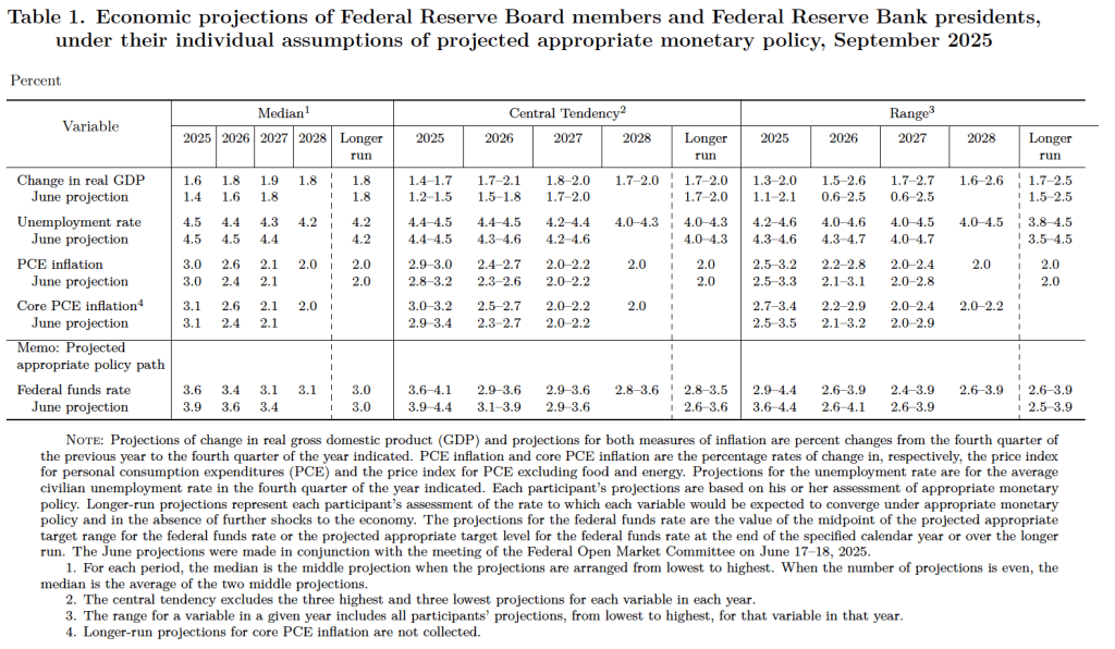
There are several aspects of these forecasts worth noting:
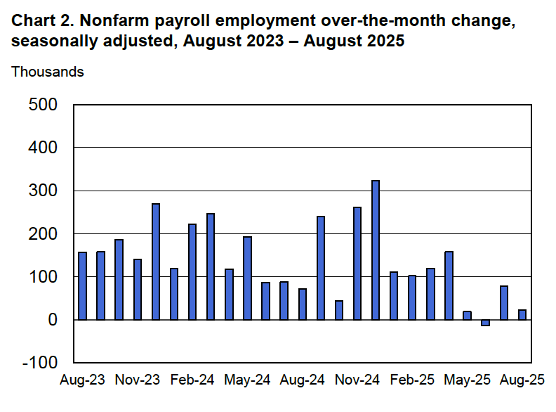
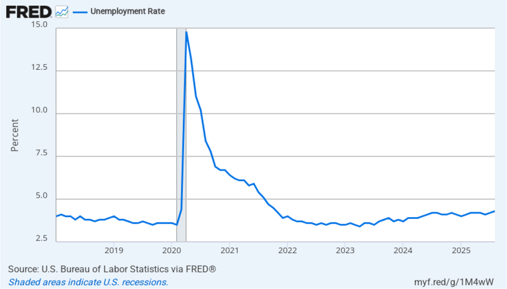
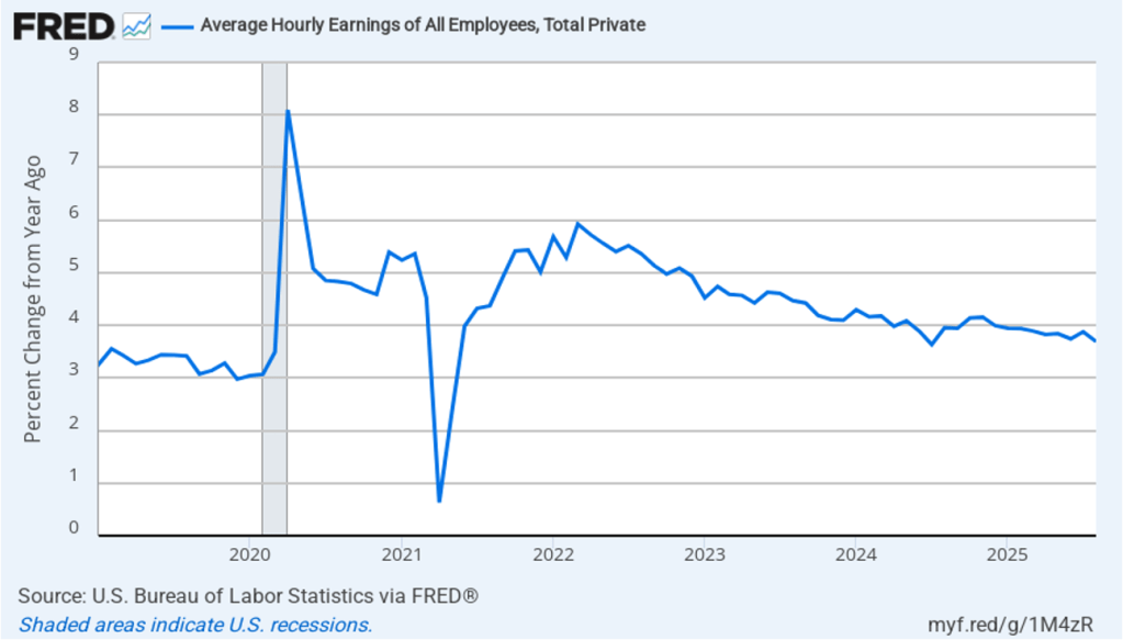
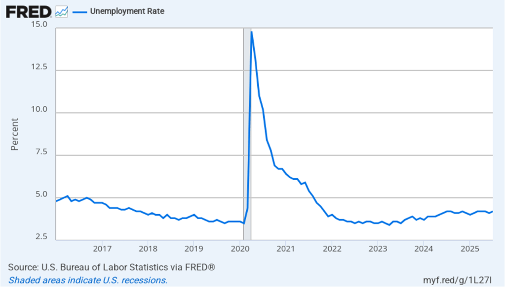
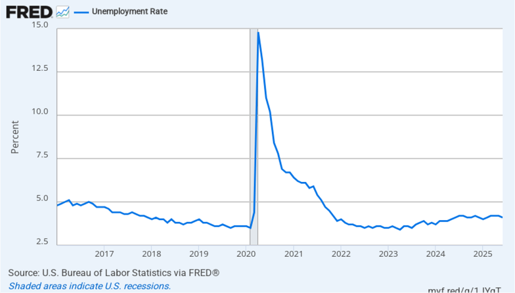
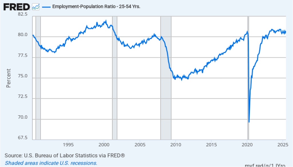
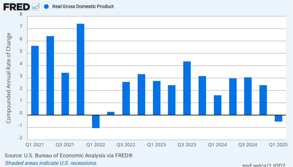
- Committee members slightly increased their forecasts of real GDP growth for each year from 2025 through 2027. Committee members also slightly decreased their forecasts of the unemployment rate in 2026 and 2027. They left their forecast of unemployment in the fourth quarter of 2025 unchanged at 4.5 percent. (The unemployment rate in August was 4.3 percent.)
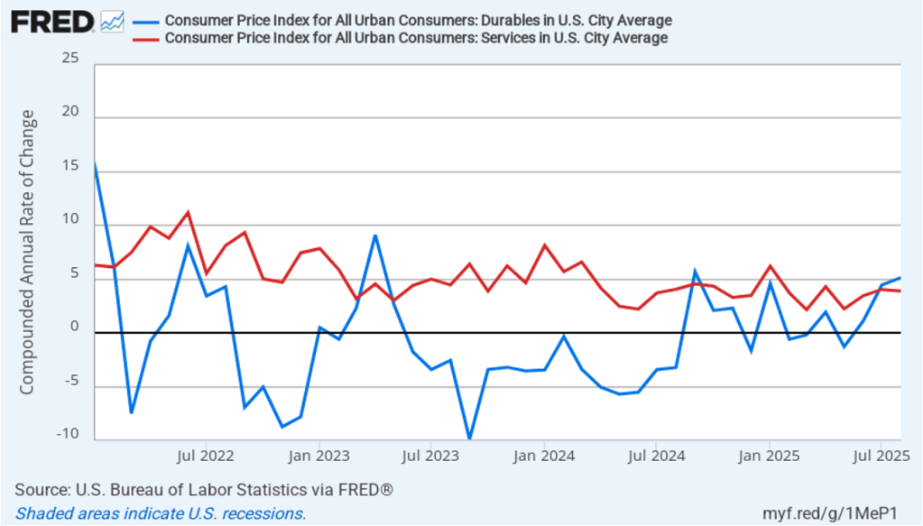
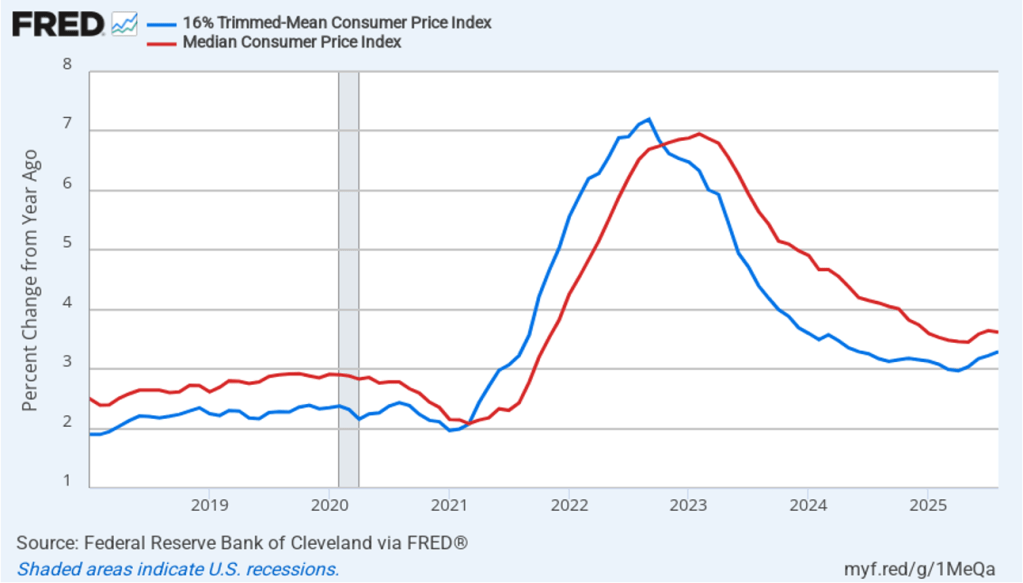
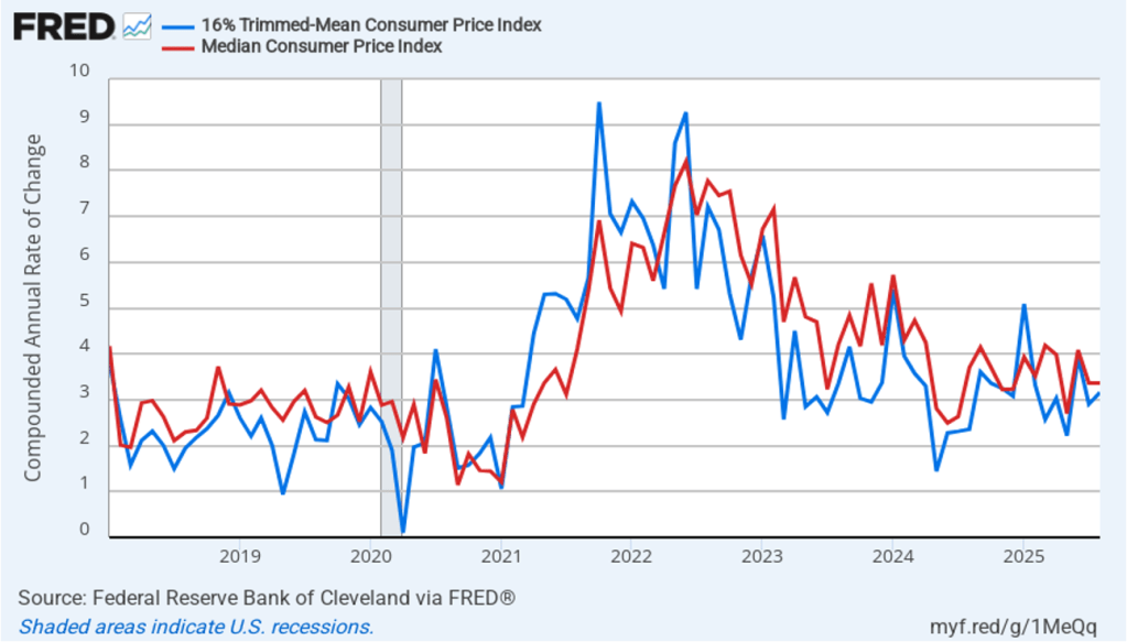
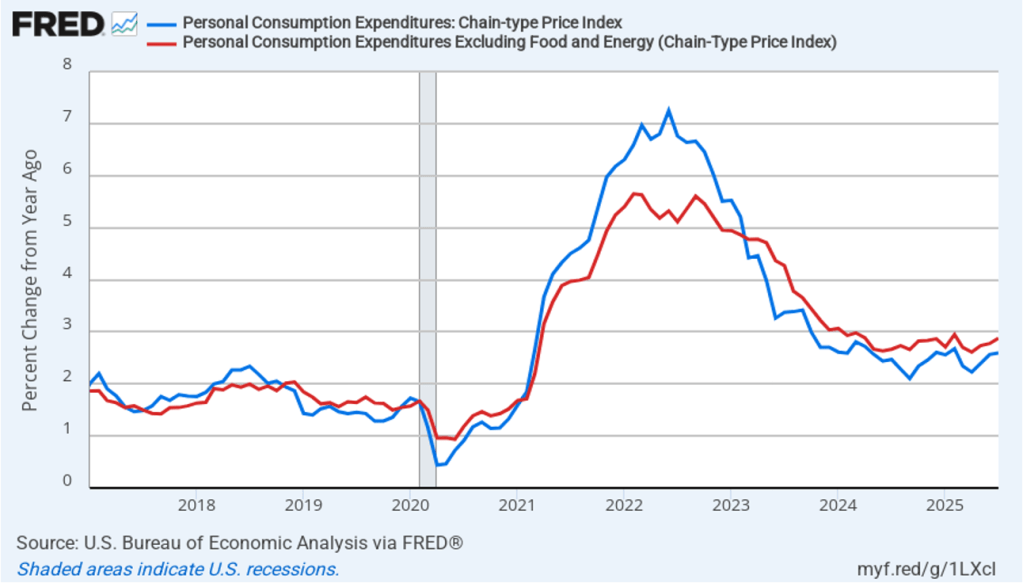
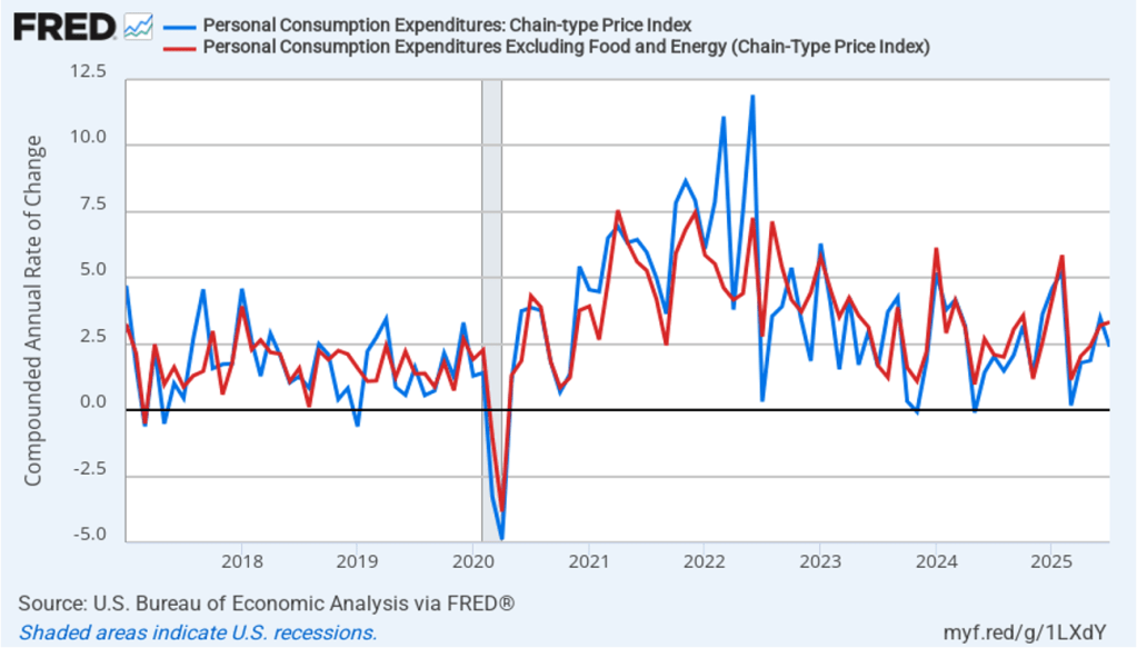
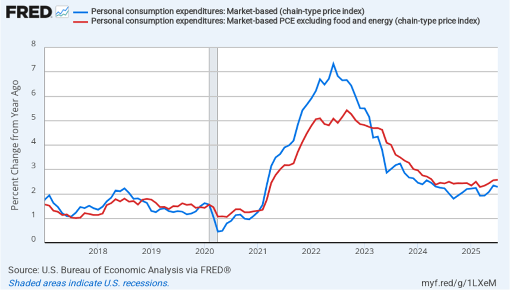
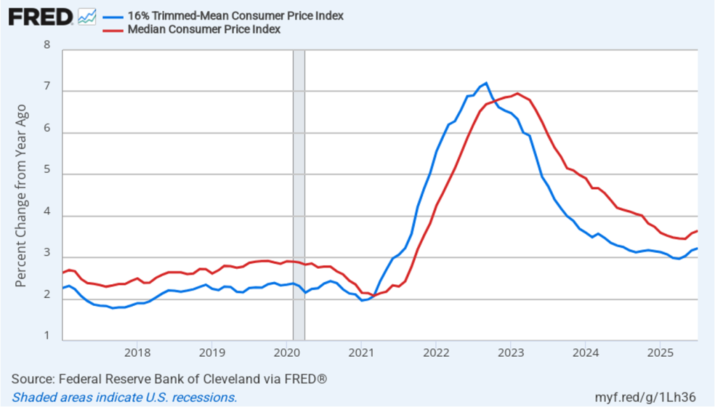
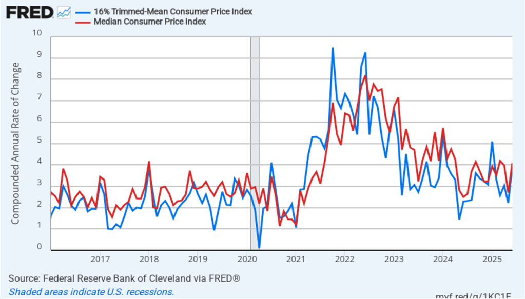
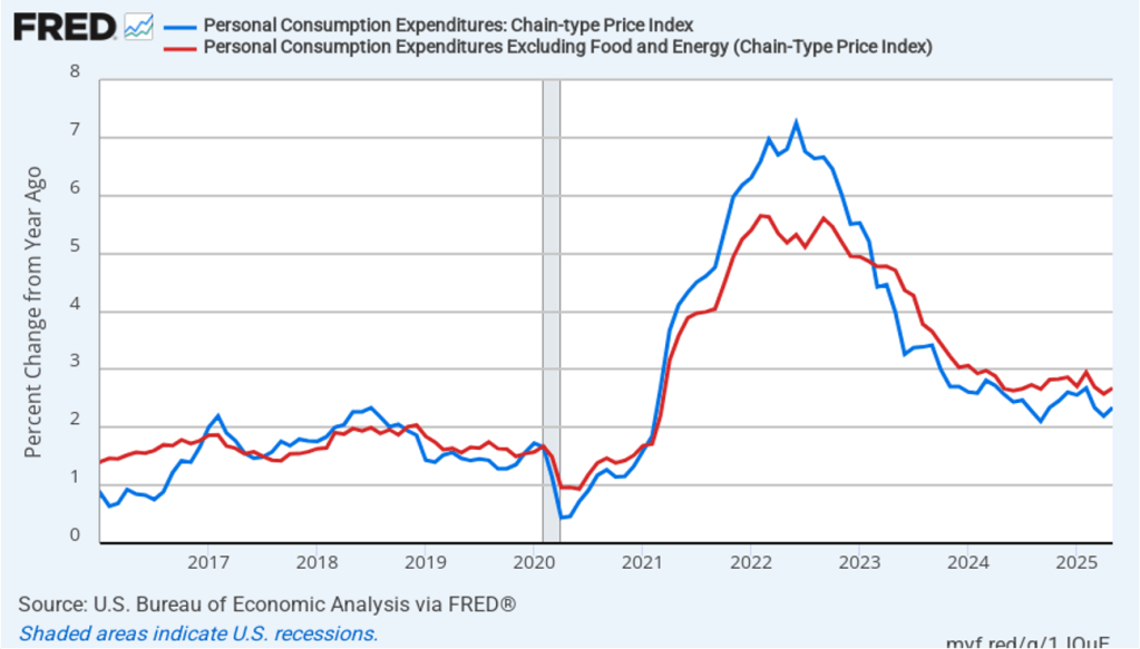
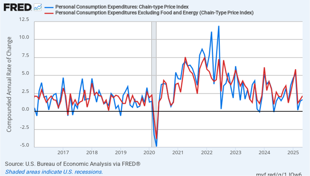
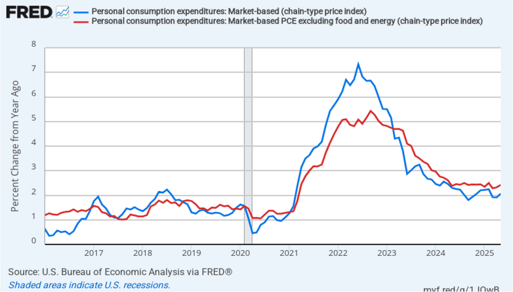
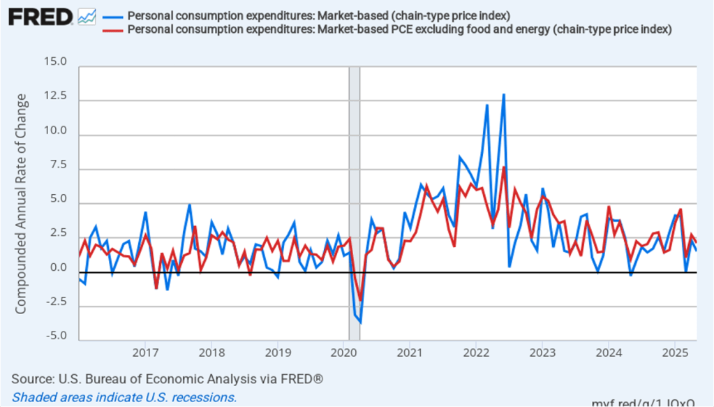
- Committee members left their forecasts for personal consumption expenditures (PCE) price inflation unchanged for 2025 and 2026, while raising their forecast for 2026 from 2.4 percent to 2.6 percent. Similarly, their forecasts of core PCE inflation were unchanged for 2025 and 2027 but increased from 2.4 percent to 2.6 percent for 2026. The committee does not expect that PCE inflation will decline to the Fed’s 2 percent annual target until 2028.
- The committee’s forecast of the federal funds rate at the end of 2025 was lowered from 3.9 percent in June to 3.6 percent today. They also lowered their forecast for federal funds rate at the end of 2026 from 3.6 percent to 3.4 pecent and at the end of 2027 from 3.4 percent to 3.1 percent.
Prior to the meeting there was much discussion in the business press and among investment analysts about the dot plot, shown below. Each dot in the plot represents the projection of an individual committee member. (The committee doesn’t disclose which member is associated with which dot.) Note that there are 19 dots, representing the 7 members of the Fed’s Board of Governors and all 12 presidents of the Fed’s district banks.
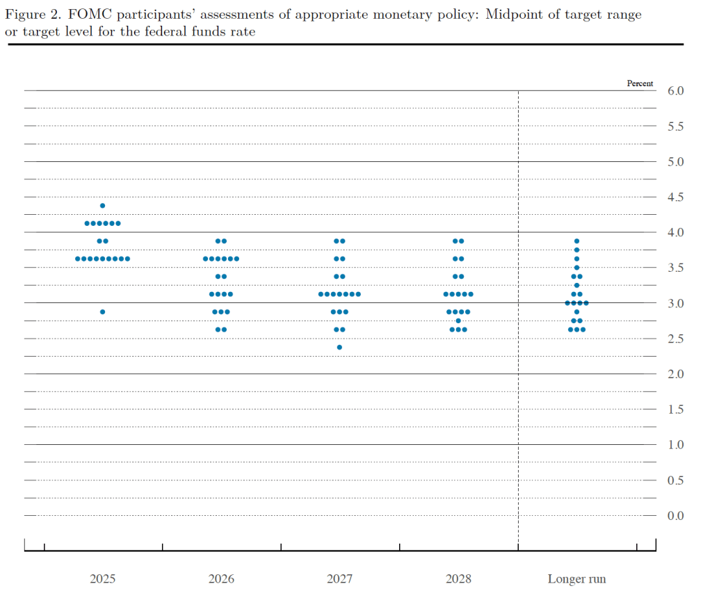
The plots on the far left of the figure represent the projections of each of the 19 members of the value of the federal funds rate at the end of 2025. Ten of the 19 members expect that the committee will cut its target range for the federal funds rate by at least 50 basis points in its two remaining meetings this year. That narrow majority makes it likely that an unexpected surge in inflation during the next few months might result in the target range being cut by only 25 basis points or not cut at all. Members of the business press and financial analysts are expecting tht the committee will implement a 25 basis point cut in each of its last two meetings this year.
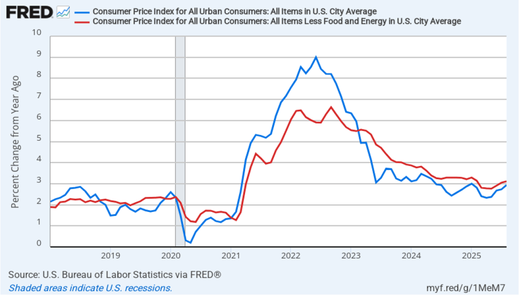
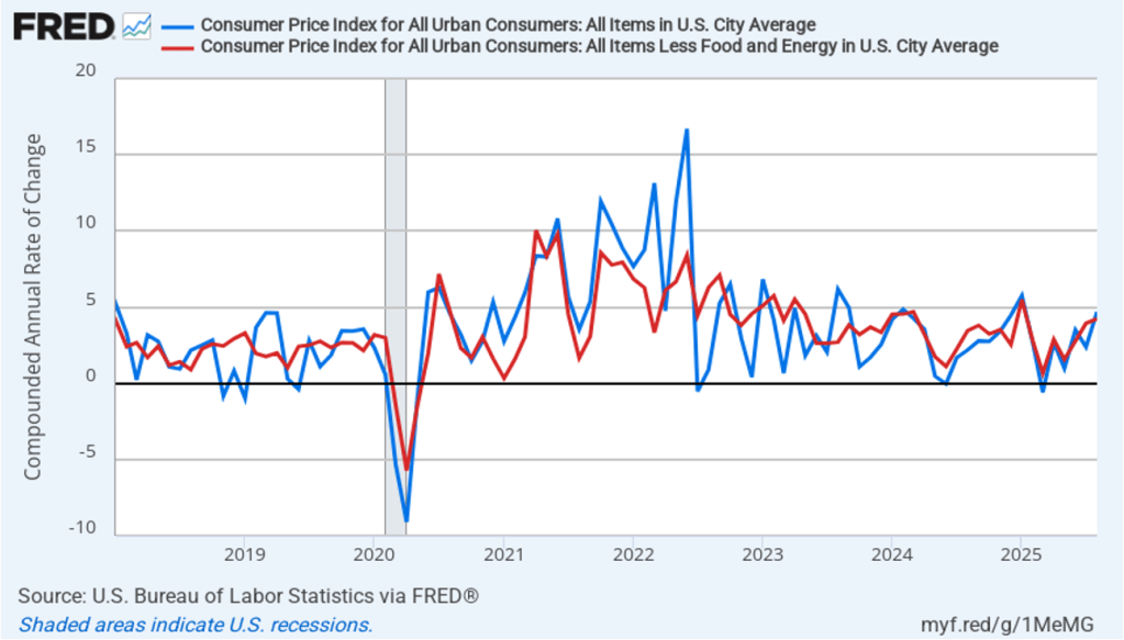
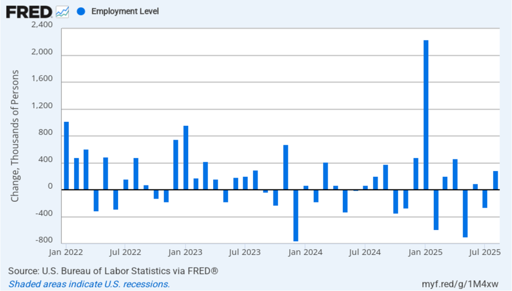
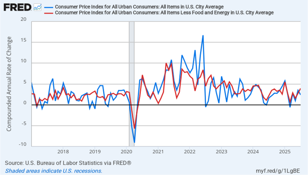
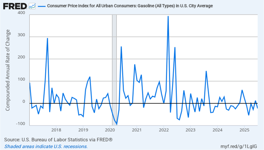
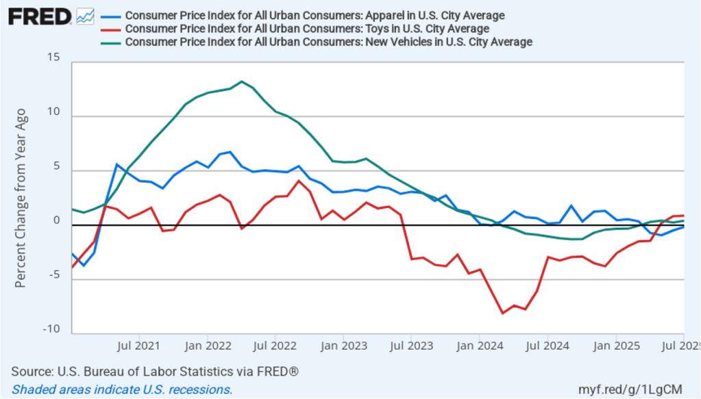
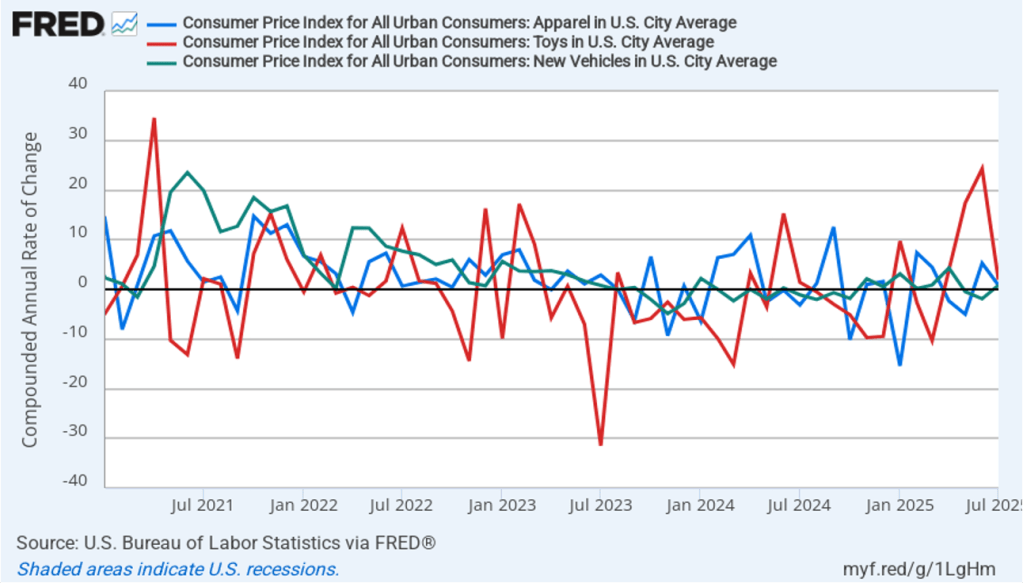
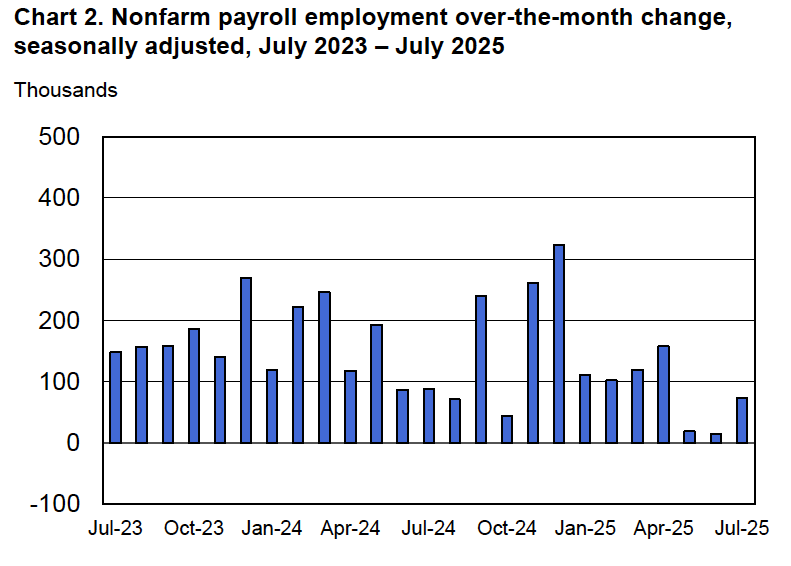
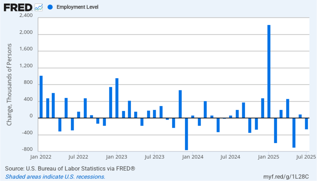
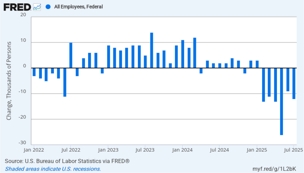
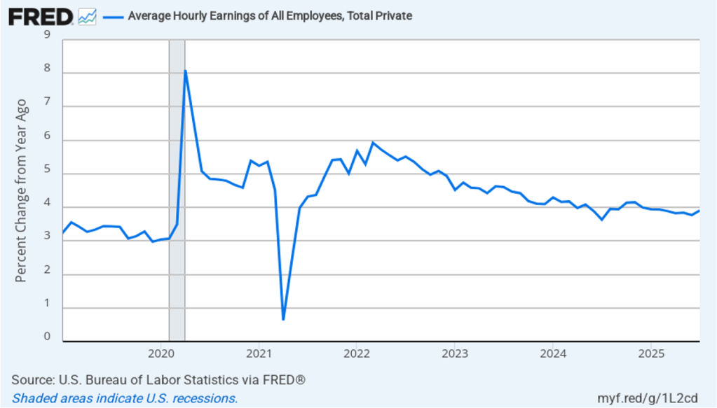
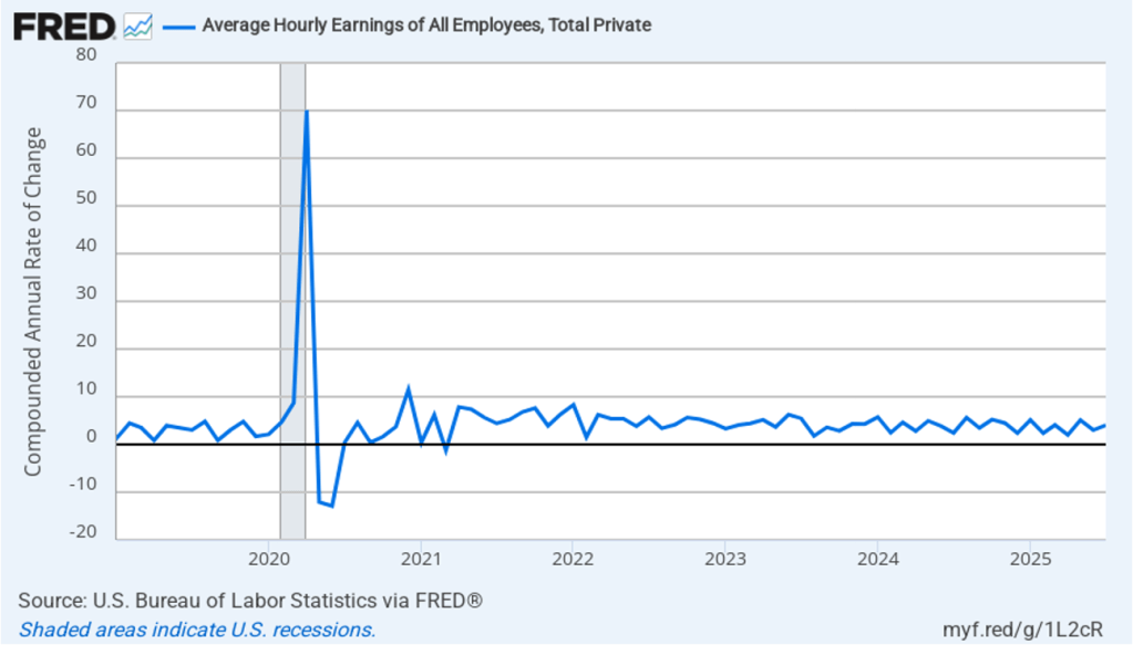
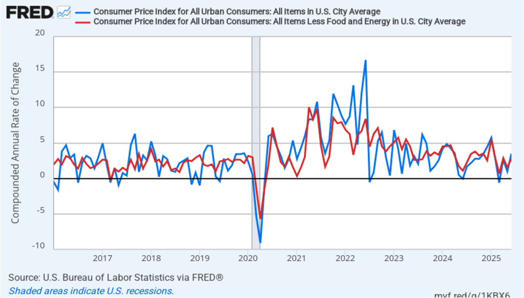
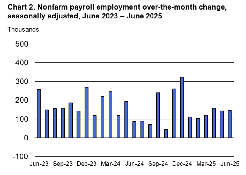
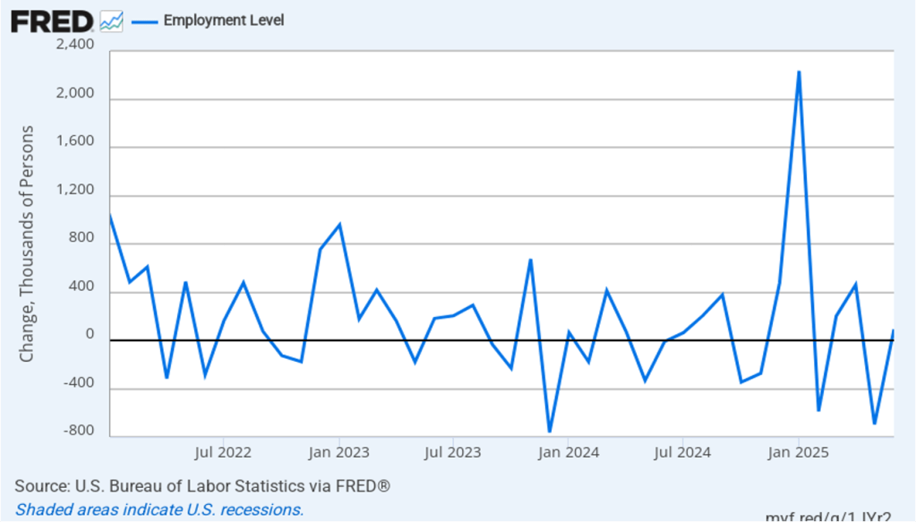
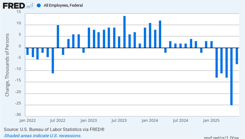
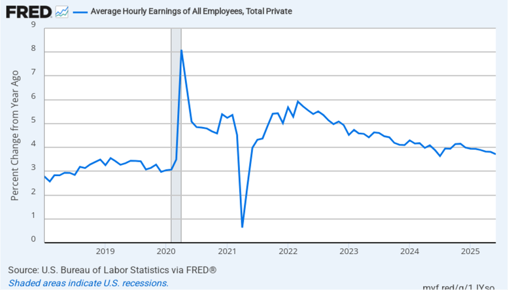
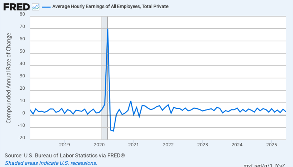
During his press conference following the meeting, Powell indicated that the recent increase in inflation was largely due to the effects of the increase in tariff rates that the Trump administration began implementing in April. (We discuss the recent data on inflation in this post.) Powell indicated that committee members expect that the tariff increases will cause a one-time increase in the price level, rather than causing a long-term increase in the inflation rate. Powell also noted recent slow growth in real GDP and employment. (We discuss the recent employment data in this blog post.) As a result, he said that the shift in the “balance of risks” caused the committee to believe that cutting the target for the federal funds rate was warranted to avoid the possibility of a significant rise in the unemployment rate.
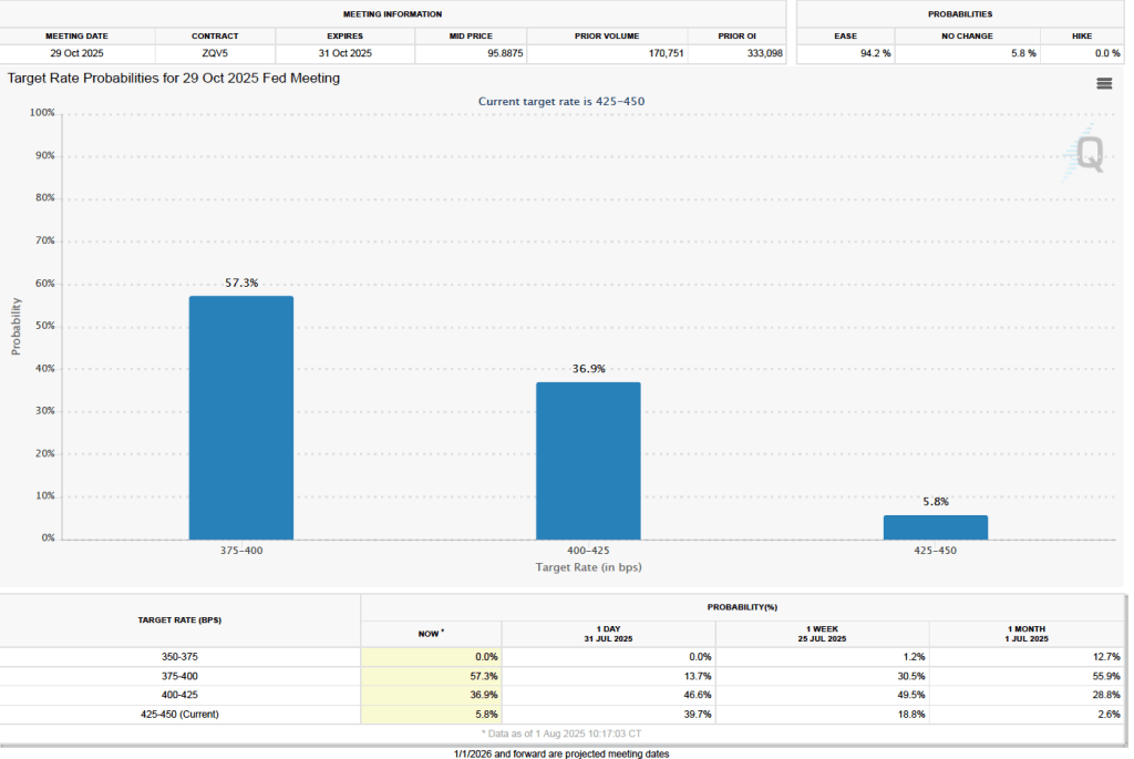
The next FOMC meeting is on October 28–29 by which time the status of Lisa Cook on the committee may have been clarified. It also seems likely that President Trump will have named the person he intends to nominate to succeed Powell as Fed chair when Powell’s term ends on May 15, 2026. (Powel’s term on the Board doesn’t end until January 31, 2028, although Fed chairs typically resign from the Board if they aren’t reappointed as chair). And, of course, additional data on inflation and unemployment will also have been released.