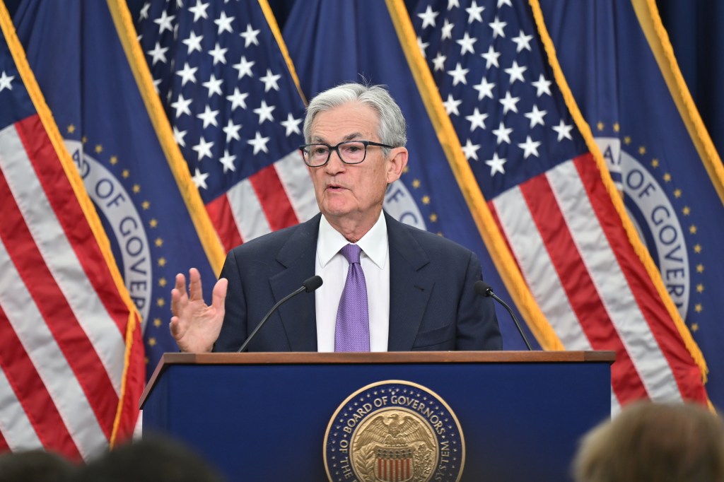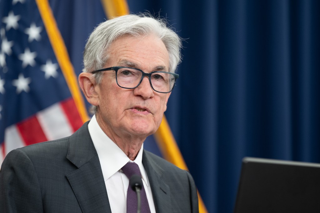
Photo from federalreserve.gov
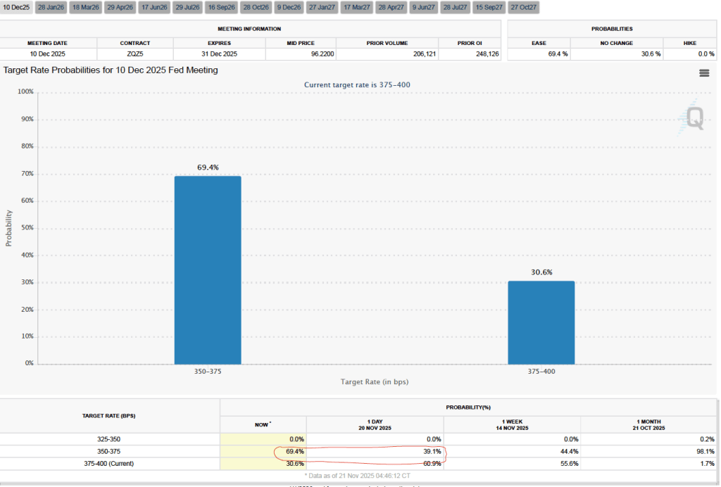
Today’s meeting of the Federal Reserve’s policymaking Federal Open Market Committee (FOMC) had the expected result with the committee deciding to lower its target for the federal funds rate from a range of 3.75 percent to 4.00 percent to a range of 3.50 percent to 3.75 percent—a cut of 25 basis points. The members of the committee voted 9 to 3 in favor of the cut. Fed Governor Stephen Miran voted against the action, preferring to lower the target range for the federal funds rate by 50 basis points. President Austan Goolsbee of the Federal Reserve Bank of Chicago and President Jeffrey Schmid of the Federal Reserve Bank of Kansas City also voted against the action, preferring to leave the target range unchanged.
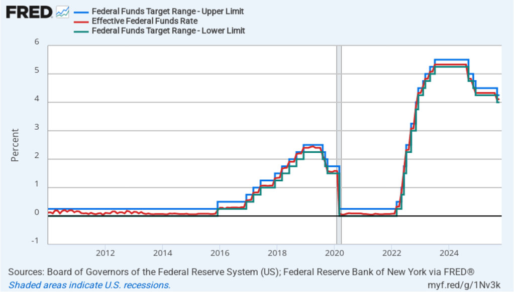
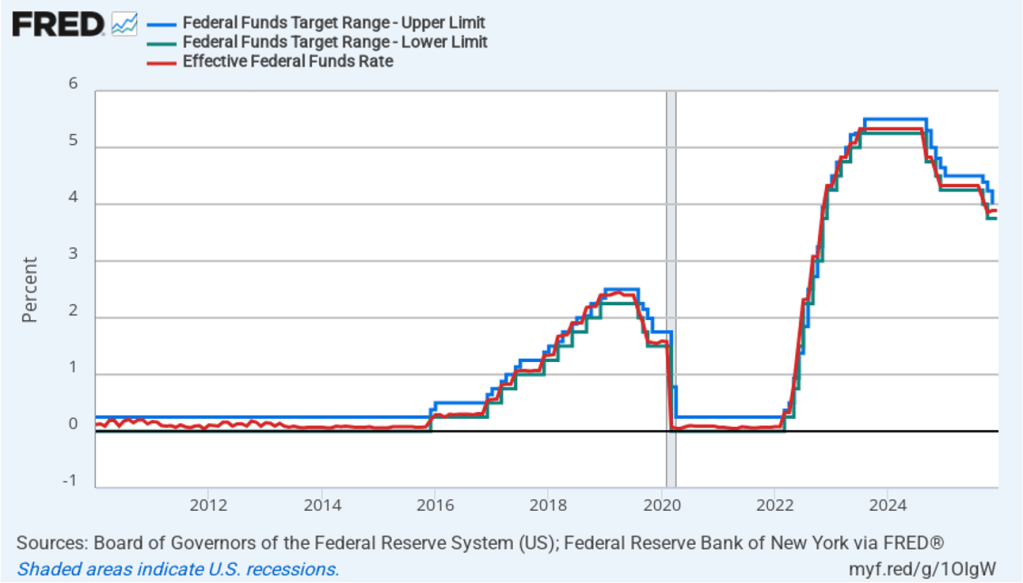
The following figure shows for the period since January 2010, the upper bound (the blue line) and the lower bound (the green line) for the FOMC’s target range for the federal funds rate, as well as the actual values for the federal funds rate (the red line). Note that the Fed has been successful in keeping the value of the federal funds rate in its target range. (We discuss the monetary policy tools the FOMC uses to maintain the federal funds rate within its target range in Macroeconomics, Chapter 15, Section 15.2 (Economics, Chapter 25, Section 25.2).)
After the meeting, the committee also released a “Summary of Economic Projections” (SEP)—as it typically does after its March, June, September, and December meetings. The SEP presents median values of the 19 committee members’ forecasts of key economic variables. The values are summarized in the following table, reproduced from the release. (Note that only 5 of the district bank presidents vote at FOMC meetings, although all 12 presidents participate in the discussions and prepare forecasts for the SEP.)
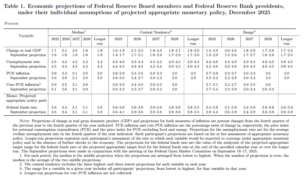
There are several aspects of these forecasts worth noting:
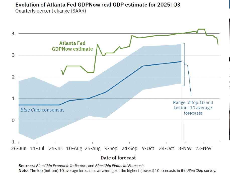
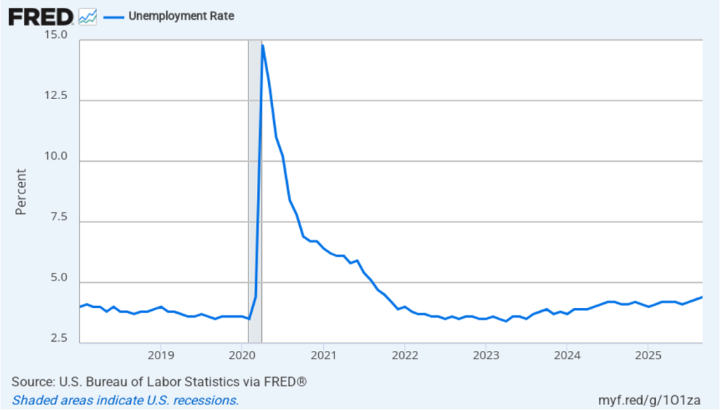
- Compared with September, the committee members increased their forecasts of real GDP growth for each year from 2025 through 2027. The increase for 2026 was substantial, from 1.8 percent to 2.3 percent, although some of this increase was attributable to the federal government shutdown causing some economic output to be shifted from 2025 to 2026. Committee members slightly decreased their forecasts of the unemployment rate in 2027. They left their forecast of the unemployment rate in the fourth quarter of 2025 unchanged at 4.5 percent.
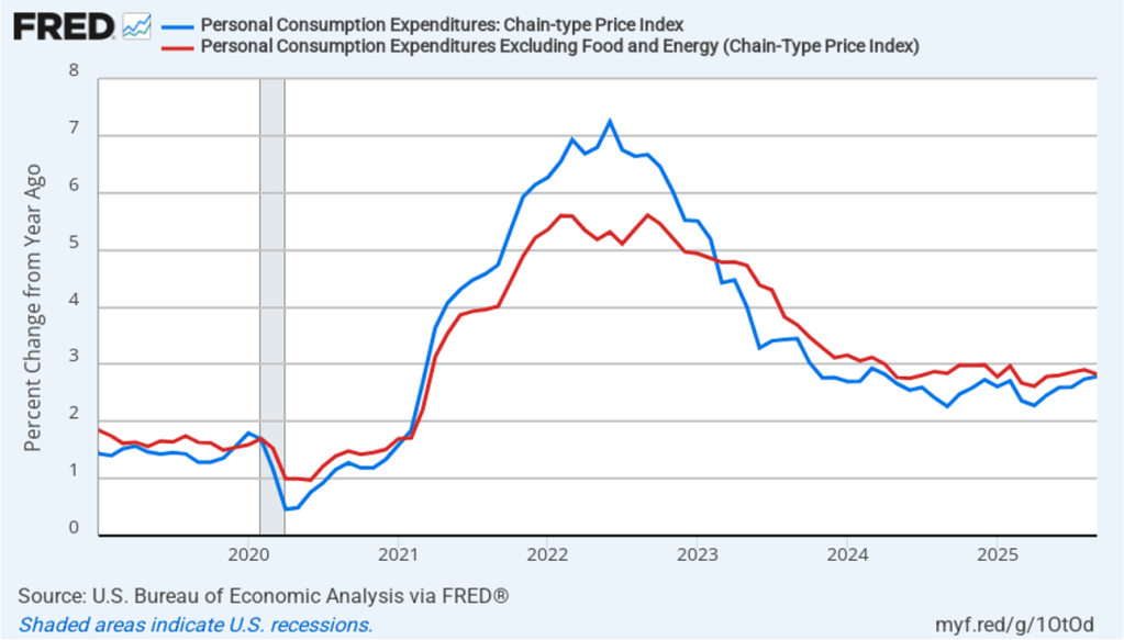
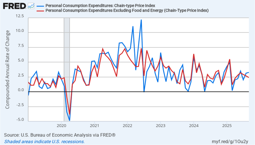
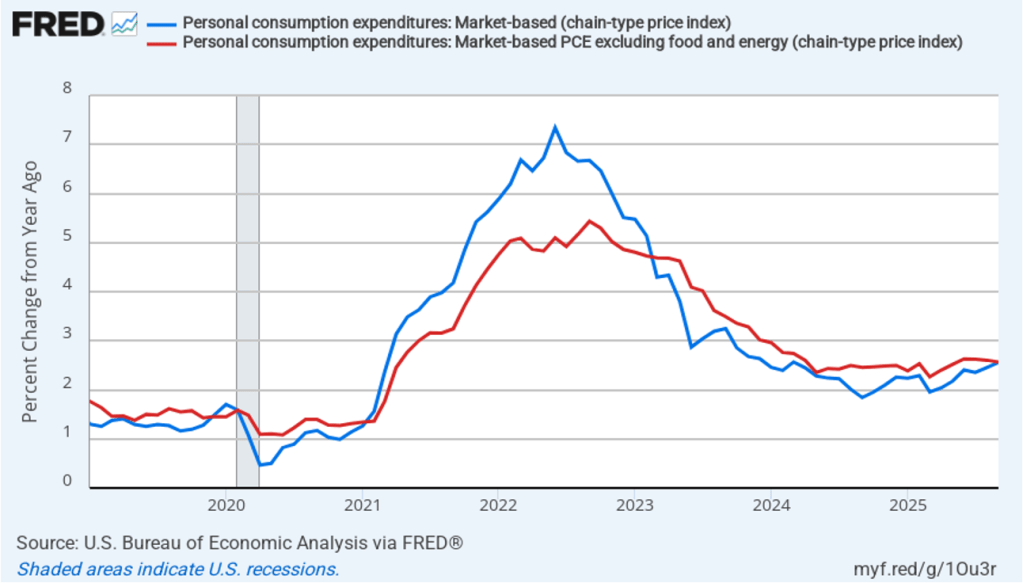
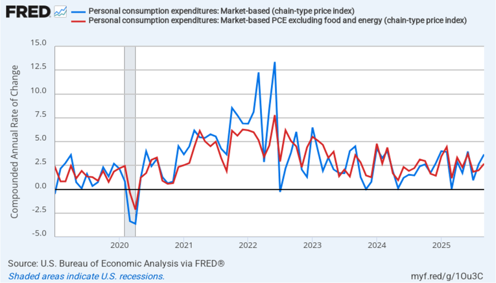
- Committee members reduced their forecasts for personal consumption expenditures (PCE) price inflation for 2025 and 2026. Similarly, their forecasts of core PCE inflation for 2025 and 2026 were also reduced. The committee does not expect that PCE inflation will decline to the Fed’s 2.0 percent annual target until 2028.
- The committee’s forecasts of the federal funds rate at the end of each year from 2025 through 2028 were unchanged.
Prior to the meeting there was much discussion in the business press and among investment analysts about the dot plot, shown below. Each dot in the plot represents the projection of an individual committee member. (The committee doesn’t disclose which member is associated with which dot.) Note that there are 19 dots, representing the 7 members of the Fed’s Board of Governors and all 12 presidents of the Fed’s district banks.
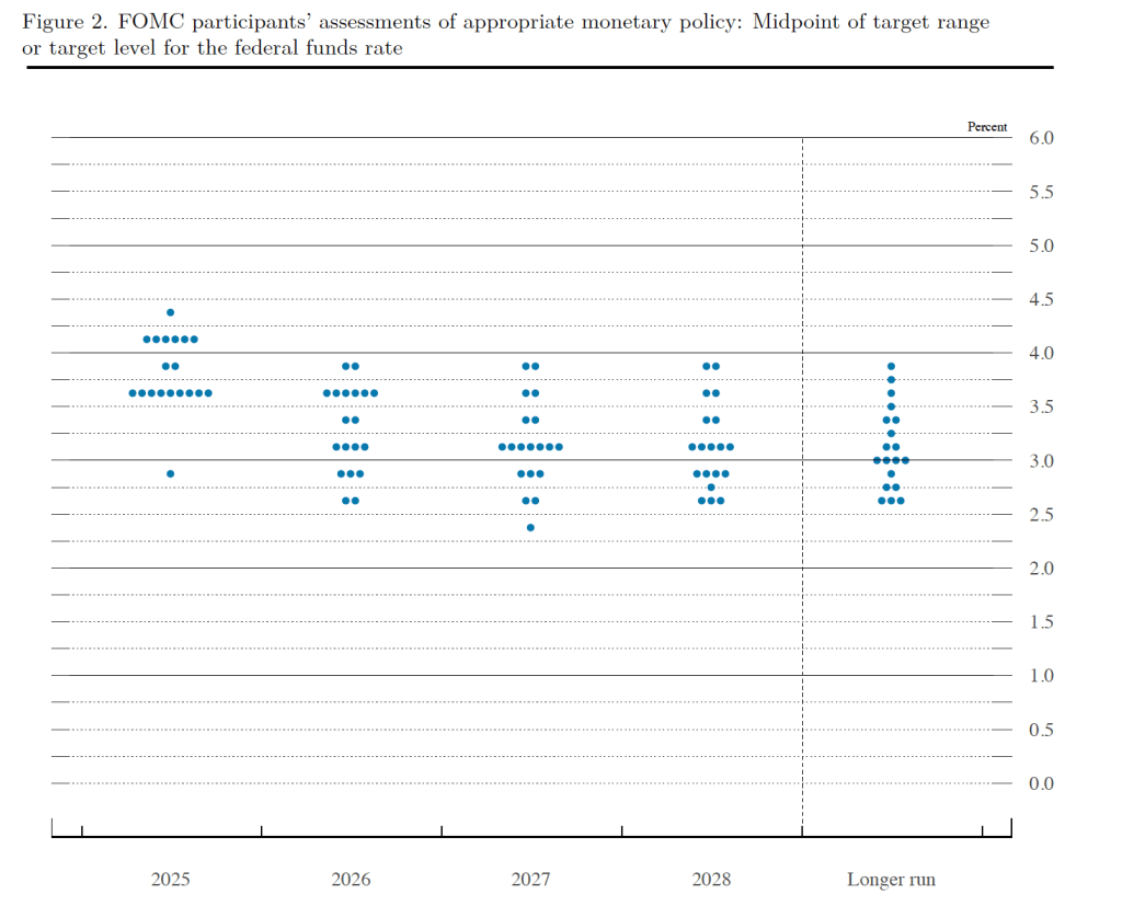
The plots on the far left of the figure represent the projections by the 19 members of the value of the federal funds rate at the end of 2025. The fact that several members of the committee preferred that the federal funds rate end 2025 above 4 percent—in other words higher than it will be following the vote at today’s meeting—indicates that several non-voting district bank presidents, beyond Goolsbee and Schmid, would have preferred to not cut the target range. The plots on the far right of the figure indicate that there is substantial disagreement among comittee members as to what the long-run value of the federal funds rate—the so-called neutral rate—should be.
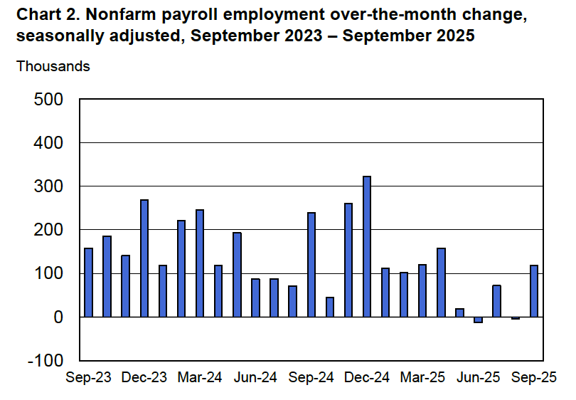
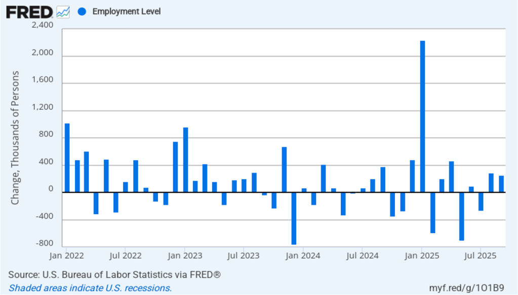
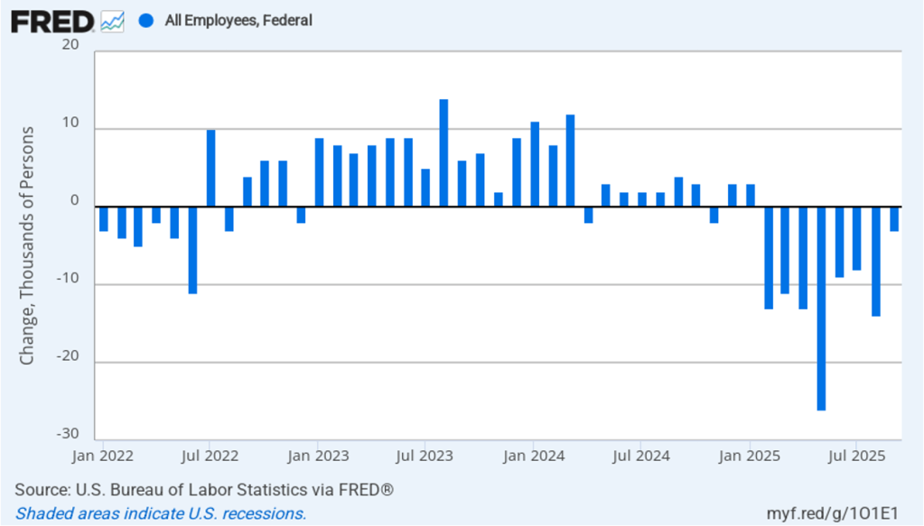
During his press conference following the meeting, Powell indicated that the increase in inflation in recent months was largely due to the effects of the increase in tariffs on goods prices. Powell indicated that committee members expect that the tariff increases will cause a one-time increase in the price level, rather than causing a long-term increase in the inflation rate. Powell also noted the recent slow growth in employment, which he noted might actually be negative once the Bureau of Labor Statistics revises the data for recent months. This slow growth indicated that the risk of unemployment increasing was greater than the risk of inflation increasing. As a result, he said that the “balance of risks” caused the committee to believe that cutting the target for the federal funds rate was warranted to avoid the possibility of a significant rise in the unemployment rate.
The next FOMC meeting is on January 27–28. By that time a significant amount of new macroeconomic data, which has not been available because of the government shutdown, will have been released. It also seems likely that President Trump will have named the person he intends to nominate to succeed Powell as Fed chair when Powell’s term ends on May 15, 2026. (Powel’s term on the Board doesn’t end until January 31, 2028, although he declined at the press conference to say whether he will serve out the remainder of his term on the Board after he steps down as chair.) In addition, it’s possible that by the time of the next meeting the Supreme Court will have ruled on whether President Trump can legally remove Governor Lisa Cook from the Board and on whether President Trump’s tariff increases this year are Constitutional.