Image created by ChatGPT
Today (December 5), the Bureau of Economic Analysis (BEA) released monthly data on the personal consumption expenditures (PCE) price index for September as part of its “Personal Income and Outlays” report. Release of the report was delayed by the federal government shutdown.
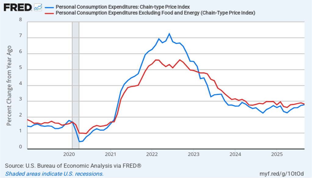
The following figure shows headline PCE inflation (the blue line) and core PCE inflation (the red line)—which excludes energy and food prices—with inflation measured as the percentage change in the PCE from the same month in the previous year. In September, headline PCE inflation was 2.8 percent, up slightly from 2.7 percent in August. Core PCE inflation in September was also 2.8 percent, down slightly from 2.9 percent in August. Both headline and core PCE inflation were equal to the forecast of economists surveyed.
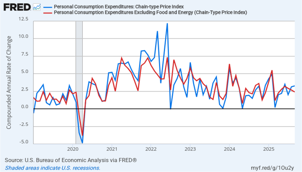
The following figure shows headline PCE inflation and core PCE inflation calculated by compounding the current month’s rate over an entire year. (The figure above shows what is sometimes called 12-month inflation, while the figure below shows 1-month inflation.) Measured this way, headline PCE inflation increased from 3.1 percent in August to 3.3 percent in September. Core PCE inflation declined from 2.7 percent in August to 2.4 percent in September. So, both 1-month and 12-month PCE inflation are telling the same story of inflation somewhat above the Fed’s target. The usual caution applies that 1-month inflation figures are volatile (as can be seen in the figure). In addition, these data are for September and likely don’t fully reflect the situation nearly two months later.
Fed Chair Jerome Powell has frequently mentioned that inflation in non-market services can skew PCE inflation. Non-market services are services whose prices the BEA imputes rather than measures directly. For instance, the BEA assumes that prices of financial services—such as brokerage fees—vary with the prices of financial assets. So that if stock prices fall, the prices of financial services included in the PCE price index also fall. Powell has argued that these imputed prices “don’t really tell us much about … tightness in the economy. They don’t really reflect that.” The following figure shows 12-month headline inflation (the blue line) and 12-month core inflation (the red line) for market-based PCE. (The BEA explains the market-based PCE measure here.)
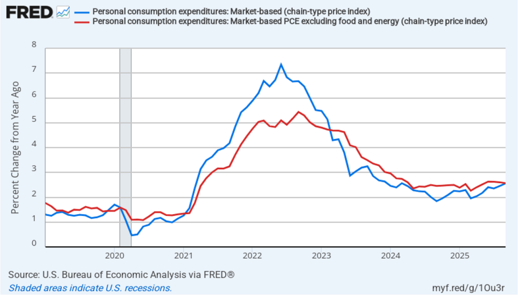
Headline market-based PCE inflation was 2.6 percent in September, up from 2.4 percent in August. Core market-based PCE inflation was 2.6 percent in September, unchanged from August. So, both market-based measures show inflation as stable but above the Fed’s 2 percent target.
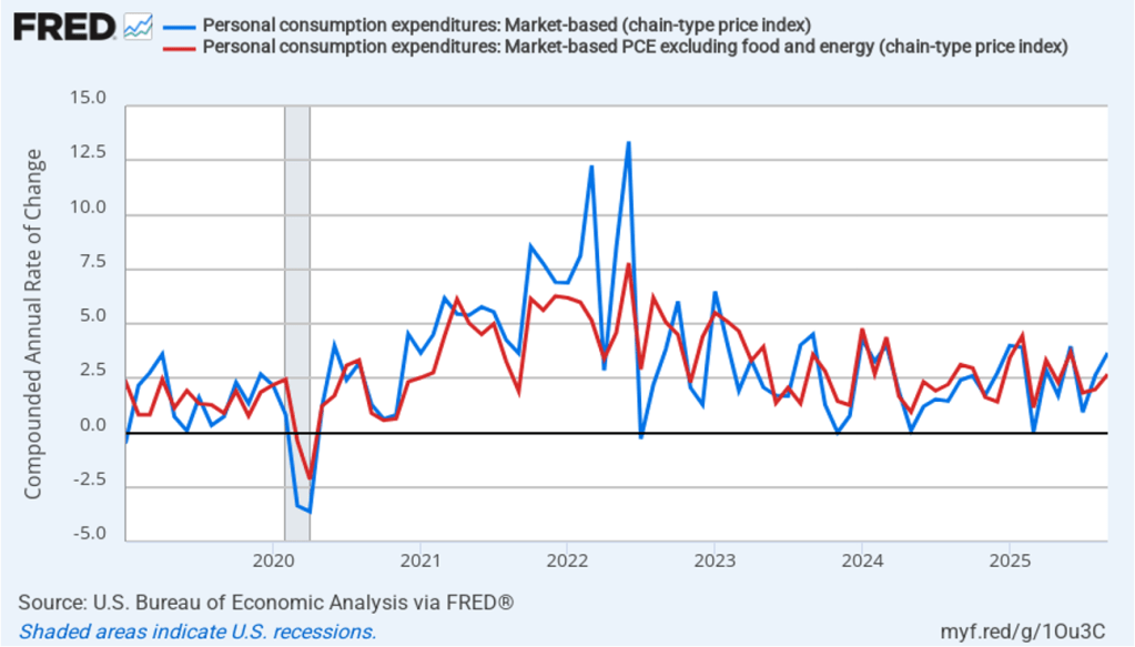
In the following figure, we look at 1-month inflation using these measures. One-month headline market-based inflation increase sharply to 3.7 percent in September from 2.6 percent in August. One-month core market-based inflation increased to 2.7 percent in September from 2.0 percent in August. As the figure shows, the 1-month inflation rates are more volatile than the 12-month rates, which is why the Fed relies on the 12-month rates when gauging how close it is coming to hitting its target inflation rate.
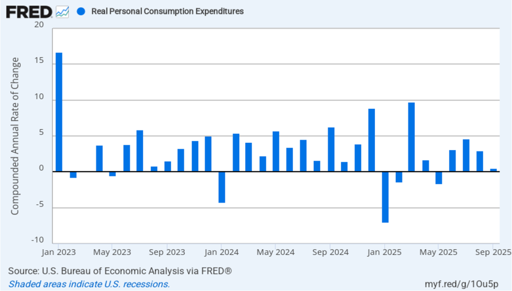
Data on real personal consumption expenditures were also included in this report. The following figure shows compound annual rates of growth of real real personal consumptions expenditures for each month since January 2023. Measured this way, the growth in real personal consumptions expenditures slowed sharply in September to 0.5 percent from 3.0 percent in August.
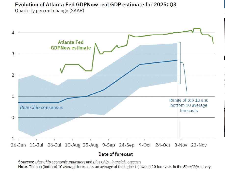
Does the slowing in consumptions spending indicate that real GDP may have also grown slowly in the third quarter of 2025? Economists at the Federal Reserve Bank of Atlanta prepare nowcasts of real GDP. A nowcast is a forecast that incorporates all the information available on a certain date about the components of spending that are included in GDP. The Atlanta Fed calls its nowcast GDPNow. As the following figure from the Atlanta Fed website shows, today the GDPNow forecast—taking into account today’s data on real personal consumption expenditures—is for real GDP to grow at an annual rate of 3.5 percent in the third quarter, which reflects continuing strong growth in other measures of output.
In a number of earlier blog posts, we discussed the policy dilemma facing the Fed. Despite the Atlanta Fed’s robust estimate of real GDP growth, there are some indications that the labor market may be weakening. For instance, earlier this week ADP estimated that private sector employment declined by 32,000 jobs in November. (We discuss ADP’s job estimates in this blog post.) As the Fed’s policy-making Federal Open Market Committee (FOMC) prepares for its next meeting on December 9–10, it has to balance guarding against a potential decline in employment with concern that inflation has not yet returned to the Fed’s 2 percent annual target.
If the committee decides that inflation is the larger concern, it is likely to leave its target range for the federal funds rate unchanged. If it decides that weakness in the labor market is the larger concern, it is likely to reduce it target range by 0.25 percentage point (25 basis points). Statements by FOMC members indicate that opinion on the committee is divided. In addition, the Trump administration has brought pressure on the committee to cut its target rate.
One indication of expectations of future changes in the FOMC’s target for the federal funds rate comes from investors who buy and sell federal funds futures contracts. (We discuss the futures market for federal funds in this blog post.) Investors’ expectations have been unusually volatile during the past two months as new macroeconomic data or new remarks by FOMC members have caused swings in the probability that investors assign to the committee cutting the target range.
As of this afternoon, investors assigned a 87.2 percent probability to the committee cutting its target range for the federal funds rate by 25 basis points to 3.50 percent to 3.75 percent at its December meeting. At the December meeting the committee will also release its Summary of Economic Projections (SEP) giving members forecasts of future values of the inflation rate, the unemployment rate, the federal funds rate, and the growth rate of real GDP. The SEP, along with Fed Chair Powell’s remarks at his press conference following the meeting, should provide additional information on the monetary policy path the committee intends to follow in the coming months.