A Brief Overview of Tariffs

Image generated by GTP-4o

A tariff is a tax a government imposes on imports. Since the end of World War II, high-income countries have only occasionally used tariffs as an important policy tool. The following figure shows how the average U.S. tariff rate, expressed as a percentage of the value of total imports, has changed in the years since 1790. The ups and downs in tariff rates reflect in part political disa-greements in Congress. Generally speaking, through the early twentieth century, members of Congress who represented areas in the Midwest and Northeast that were home to many manufacturing firms favored high tariffs to protect those industries from foreign competition. Members of Congress from rural areas opposed tariffs, because farmers were primarily exporters who feared that foreign governments would respond to U.S. tariffs by imposing tariffs on U.S. agricultural exports. From the pre-Civil War period until after World War II the Republicans Party generally favored high tariffs and the Democratic Party generally favored low tariffs, reflecting the economic interests of the areas the parties represented in Congress. (Note: Because the tariffs that the Trump Administration will end up imposing are still in flux, the value for 2025 in the figure is only a rough estimate.)

By the end of World War II in 1945, government officials in the United States and Europe were looking for a way to reduce tariffs and revive international trade. To help achieve this goal, they set up the General Agreement on Tariffs and Trade (GATT) in 1948. Countries that joined the GATT agreed not to impose new tariffs or import quotas. In addition, a series of multilateral negotiations, called trade rounds, took place, in which countries agreed to reduce tariffs from the very high levels of the 1930s. The GATT primarily covered trade in goods. A new agreement to cover services and intellectual property, as well as goods, was eventually negotiated, and in January 1995, the GATT was replaced by the World Trade Organization (WTO). In 2025, 166 countries are members of the WTO.

As a result of U.S. participation in the GATT and WTO, the average U.S. tariff rate declined from nearly 20% in the early 1930s to 1.8% in 2018. The first Trump Administration increased tariffs beginning in 2018, raising the average tariff rate to 2.5%. (The Biden Administration continued most of the increases.) In 2025, the second Trump Administration’s substantial increases in tariffs raised the average tariff rate to the highest level since the 1940s.

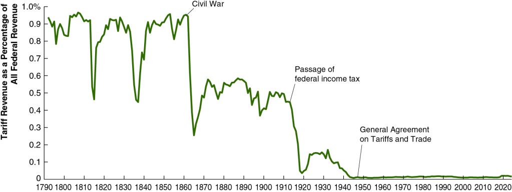
Until the enactment in 1913 of the 16th Amendment to the U.S. Constitution, which allowed for a federal income tax, tariffs were an important source of revenue to the federal government. As the following figure shows, in the early years of the United States, more than 90% of federal government revenues came from the tariff. As tariff rates declined and federal income and payroll taxes increased, tariffs declined to only 2% of federal government revenue. It’s unclear yet how much tariff’s share of federal government revenue will rise as a result of the Trump Administration’s tariff increases.
The effect of tariff increases on the U.S. economy are complex and depend on the details of which tariffs are increased, by how much they are increased, and whether foreign governments raise their tariffs on U.S. exports in response to U.S. tariff increases. We can analyze some of the effects of tariffs using the basic aggregate demand and aggregate supply model that we discuss in Macroeconomics, Chapter 13 (Economics, Chapter 23). We need to keep in mind in the following discussion that small increases in tariffs rates—such as those enacted in 2018—will likely have only small effects on the economy given that net exports are only about 3% or U.S. GDP.

An increase in tariffs intended to protect domestic industries can cause the aggregate demand curve to shift to the right if consumers switch spending from imports to domestically produced goods, thereby increasing net exports. But this effect can be partially or wholly offset if trading partners retaliate by increasing tariffs on U.S. exports. When Congress passed the Smoot-Hawley Tariff in 1930, which raised tariff rates to historically high levels, retaliation by U.S. trading partners contributed to a sharp decline in U.S. exports during the early 1930s.

International trade can increase a country’s production and income by allowing a country to specialize in the goods and services in which it has a comparative advantage. Tariffs shift a country’s allocation of labor, capital, and other resources away from producing the goods and services it can produce most efficiently and toward producing goods and services that other countries can produce more efficiently. The result of this misallocation of resources is to reduce the productive capacity of the country, shifting the long-run aggregate supply curve (LRAS) to the left.

Tariffs raise the prices of U.S. imports. This effect can be partially offset because tariffs increase the demand for U.S. dollars relative to trading partners’ currencies, increasing the dollar exchange rate. Because a tariff effectively acts as a tax on imports, like other taxes its incidence—the division of the burden of the tax between sellers and buyers—depends partly on the price elasticity of demand and the price elasticity of supply, which vary across the goods and services on which tariffs are imposed. (We discuss the effects of demand and supply elasticity on the incidence of a tax in Microeconomics, Chapter 17, Section 17.3.)

About two-thirds of U.S. imports are raw materials, intermediate goods, or capital goods, all of which are used as inputs by U.S. firms. For example, many cars assembled in the United States contain imported parts. The popular Ford F-Series pickup trucks are assembled in the United States, but more than two-thirds of the parts are imported from other countries. That fact indicates that the automobile industry is one of many U.S. industries that depend on global supply chains that can be disrupted by tariffs. Because tariffs on imported raw materials, parts and other intermediate goods, and capital goods increase the production costs of U.S. firms, tariffs reduce the quantity of goods these firms will produce at any given price. In terms of the aggregate demand and aggregate supply model , a large unexpected increase in tariffs results in an aggregate supply shock to the economy, shifting the short-run aggregate supply curve (SRAS) to the left.

Our thanks to Fernando Quijano for preparing the two figures.
The FOMC Leaves Its Target for the Federal Funds Rate Unchanged, while Noting an Increase in Economic Uncertainty

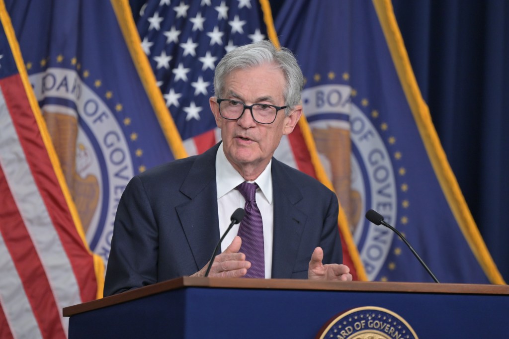
Fed Chair Jerome Powell speaking at a press conference following a meeting of the FOMC (photo from federalreserve.gov)

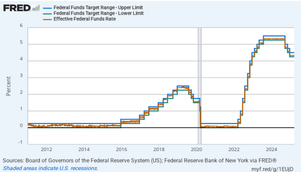
As they had before their previous meeting, members of the Fed’s Federal Open Market Committee (FOMC) had signaled that the committee was likely to leave its target range for the federal funds rate unchanged at 4.25 percent to 4.50 percent at its meeting today (March 19). In a press conference following the meeting, Fed Chair Jerome Powell noted that the FOMC was facing significant policy uncertainty:

“Looking ahead, the new Administration is in the process of implementing significant policy changes in four distinct areas: trade, immigration, fiscal policy, and regulation…. While there have been recent developments in some of these areas, especially trade policy, uncertainty around the changes and their effects on the economic outlook is high…. We do not need to be in a hurry to adjust our policy stance, and we are well positioned to wait for greater clarity.”

The next scheduled meeting of the FOMC is May 6–7. It seems likely that the committee will also keep its target rate constant at that meeting. Although at his press conference, Powell noted that “Policy is not on a preset course. As the economy evolves, we will adjust our policy stance in a manner that best promotes our maximum employment and price stability goals.” The statement the committee released after the meeting showed that the decision to leave the target rate unchanged was unanimous.

The following figure shows, for the period since January 2010, the upper bound (the blue line) and lower bound (the green line) for the FOMC’s target range for the federal funds rate and the actual values of the federal funds rate (the red line) during that time. Note that the Fed is successful in keeping the value of the federal funds rate in its target range. (We discuss the monetary policy tools the FOMC uses to maintain the federal funds rate in its target range in Macroeconomics, Chapter 15, Section 15.2 (Economics, Chapter 25, Section 25.2).)

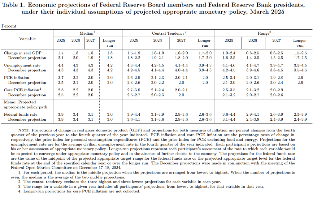
After the meeting, the committee also released a “Summary of Economic Projections” (SEP)—as it typically does after its March, June, September, and December meetings. The SEP presents median values of the 18 committee members’ forecasts of key economic variables. The values are summarized in the following table, reproduced from the release.
There are several aspects of these forecasts worth noting:

  1. Committee members reduced their forecast of real GDP growth for 2025 from 2.1 percent in December to 1.7 percent today. Committee members also slightly increased their forecast of the unemployment rate at the end of 2025 from 4.3 percent to 4.4 percent. (The unemployment rate in February was 4.1 percent.)
  2. Committee members now forecast that personal consumption expenditures (PCE) price inflation will be 2.7 percent at the end of 2025. In December, they had forecast that it would 2.5 percent. Similarly, their forecast of core PCE inflation increased from 2.5 percent to 2.8 percent. The committee does not expect that PCE inflation will decline to the Fed’s 2 percent annual target until 2027.
  3. The committee’s forecast of the federal funds rate at the end of 2025 was unchanged at 3.9 percent. The federal funds rate today is 4.33 percent, which indicates that committee members expect to make two 0.25 percentage point (25 basis points) cuts in their target for the federal funds rate this year. Investors are similarly forecasting two 25 basis point cuts.
During his press conference, Powell indicated that a significant part of the increase in goods inflation during the first two months of the year was likely due to tariffs, although the Fed’s staff was unable to make a precise estimate of how much. Economists generally believe that tariffs cause one-time increases in the price level, rather than persistent inflation. Powell was asked during the press conference whether the FOMC was likely to “look through”—that is, not respond—to the tariffs. Powell replied that it was too early to make that decision, but that: “If there’s an inflation that’s going to go away on its own, it’s not the correct response to tighten policy.”
Powell noted that although surveys show that businesses and consumers expect an increase in inflation, over the long run, expectations are that the inflation rate will return to the Fed’s 2 percent annual target. In that sense, Powell said that expectations of inflation remain “well anchored.”

Barring a sharp slowdown in the growth of real GDP, a significant rise in the unemployment rate, or a significant rise in the inflation rate, the FOMC seems likely to leave its target for the federal funds rate unchanged over the next few months.

CPI Inflation Is Lower than Expected, but Still above Target

Photo courtesy of Lena Buonanno.

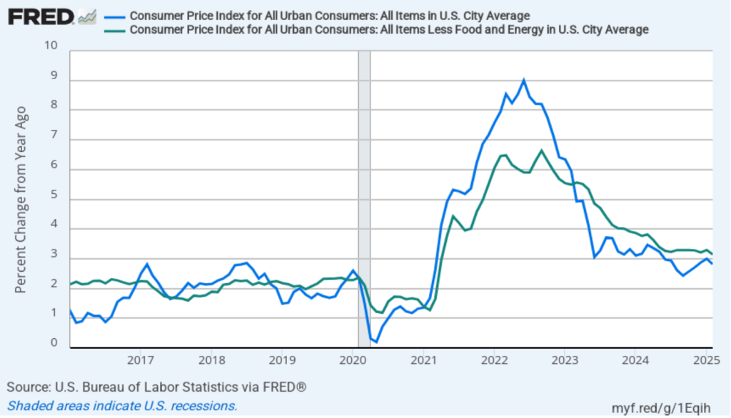
Today (March 12), the Bureau of Labor Statistics (BLS) released its monthly report on the consumer price index (CPI). The following figure compares headline inflation (the blue line) and core inflation (the green line).

  • The headline inflation rate, which is measured by the percentage change in the CPI from the same month in the previous year, was 2.8 percent in February—down from 3.0 percent in January. 
  • The core inflation rate, which excludes the prices of food and energy, was 3.1 percent in February—down from 3.3 percent in January. 

Both headline inflation and core inflation were slightly below what economists surveyed had expected.

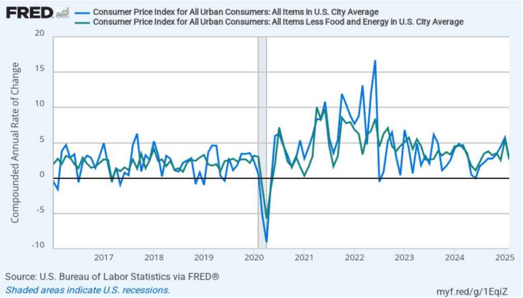
In the following figure, we look at the 1-month inflation rate for headline and core inflation—that is the annual inflation rate calculated by compounding the current month’s rate over an entire year. Calculated as the 1-month inflation rate, headline inflation (the blue line) fell sharply from 5.7 percent in February to 2.6 percent in January. Core inflation (the green line) decreased from 5.5 percent in January to 2.8 percent in January.

Overall, considering 1-month and 12-month inflation together, the most favorable news is the sharp decline in both the headline and the core 1-month inflation rats. But inflation is still running ahead of the Fed’s 2 percent annual inflation target.

Of course, it’s important not to overinterpret the data from a single month. The figure shows that 1-month inflation is particularly volatile. Also note that the Fed uses the personal consumption expenditures (PCE) price index, rather than the CPI, to evaluate whether it is hitting its 2 percent annual inflation target.

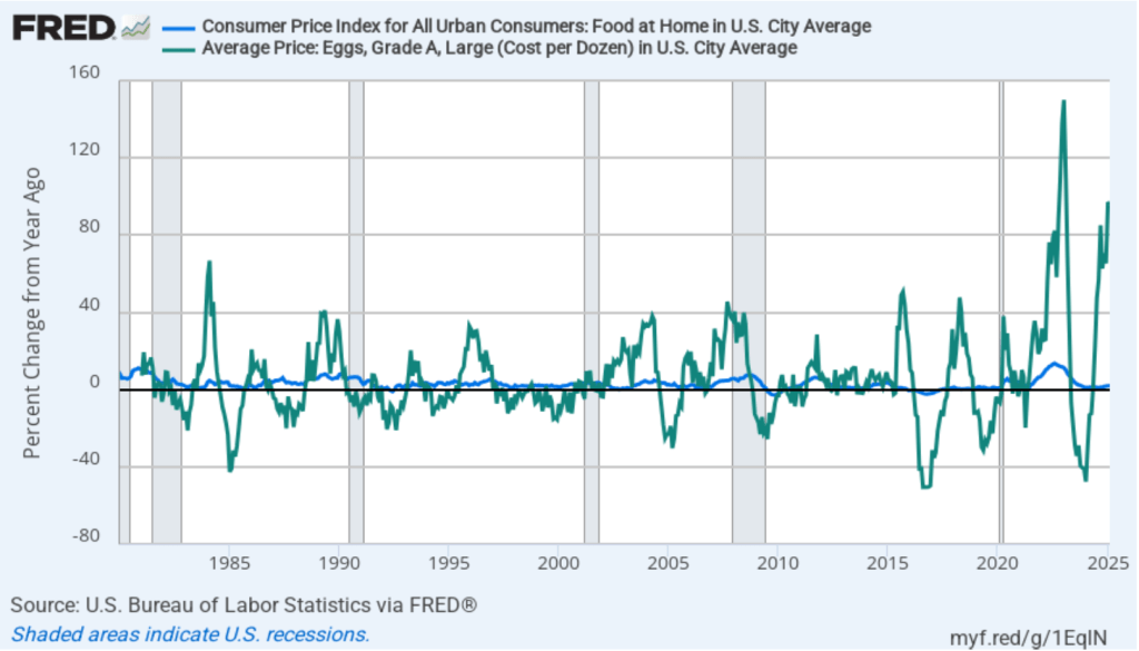
There’s been considerable discussion in the media about continuing inflation in grocery prices. In the following figure the blue line shows inflation in the CPI category “food at home,” which is primarily grocery prices. Inflation in grocery prices was 1.8 percent in February and has been below 2 percent every month since November 2023. Although on average grocery price inflation has been low, there have been substantial increases in the prices of some food items. For instance, egg prices—shown by the green line—increased by 96.8 percent in February. But, as the figure shows, egg prices are usually quite volatile month-to-month, even when the country is not dealing with an epidemic of bird flu.

To better estimate the underlying trend in inflation, some economists look at median inflation and trimmed mean inflation.

  • Median inflation is calculated by economists at the Federal Reserve Bank of Cleveland and Ohio State University. If we listed the inflation rate in each individual good or service in the CPI, median inflation is the inflation rate of the good or service that is in the middle of the list—that is, the inflation rate in the price of the good or service that has an equal number of higher and lower inflation rates. 
  • Trimmed-mean inflation drops the 8 percent of goods and services with the highest inflation rates and the 8 percent of goods and services with the lowest inflation rates. 

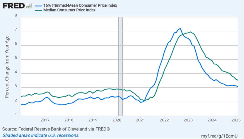
The following figure shows that 12-month trimmed-mean inflation (the blue line) was 3.1 percent in February, unchanged from January. Twelve-month median inflation (the green line) declined slightly from 3.6 percent in January to 3.5 percent in February.

The following figure shows 1-month trimmed-mean and median inflation. One-month trimmed-mean inflation fell from 5.1 percent in January to 3.3. percent in February. One-month median inflation from 3.9 percent in January to 3.5 percent in February. These data provide confirmation that (1) CPI inflation at this point is likely running higher than a rate that would be consistent with the Fed achieving its inflation target, and (2) inflation slowed somewhat from January to February.

What are the implications of this CPI report for the actions the FOMC may take at its next several meetings? The major stock market indexes rose sharply at the beginning of trading this morning, but then swung back and forth between losses and gains. Inflation being lower than expected may have increased the probability that the FOMC will cut its target for the federal funds rate sooner rather than later. Lower inflation and lower interest rates would be good news for stock prices. But investors still appear to be worried about the extent to which a trade war might both slow economic growth and increase the price level.

Investors who buy and sell federal funds futures contracts still do not expect that the FOMC will cut its target for the federal funds rate at its next two meetings. (We discuss the futures market for federal funds in this blog post.) Today, investors assigned only a 1 percent probability that the Fed’s policymaking Federal Open Market Committee (FOMC) will cut its target from the current 4.25 percent to 4.50 percent range at its meeting next week. Investors assigned a probability of 33.3 percent that the FOMC would cut its target after its meeting on May 6–7. Investors today assigned a probability of 78.6 percent that the committee will cut its target after its meeting on June 17–18. That probability has fallen slightly over the past week.

At his press conference after next Wednesday’s FOMC meeting, Fed Chair Jerome Powell will give his thoughts on the current economic situation.

Glenn on the Importance of Research

An image generated by GTP-4o illustrating research.

This opinion column by Glenn appeared in the Financial Times on March 10.

The Trump administration has wisely emphasised raising America’s rate of economic growth. But growth doesn’t just happen. It is the byproduct of innovation both radical (think of the emergence of generative artificial intelligence) and gradual (such as improvements in manufacturing processes or transport). Many economic factors influence innovation, but research and development is key. While this can be privately or publicly funded, the latter can support basic research with spillovers to many companies and applications.

Therein lies the rub: the new administration’s growth agenda is joined by a significant effort to reduce government spending, spearheaded by the so-called Department of Government Efficiency. Some spending restraint can enhance growth by reducing interest rates or reallocating funds towards more investment-oriented activities. But cuts to R&D, as the administration is advocating at the National Institutes of Health (NIH), National Science Foundation (NSF), Department of Energy (DoE) and NASA, are counter-productive. They will limit innovation and growth.

The link between R&D and productivity growth has a long pedigree in economics and has generally been acknowledged by US policymakers. In the mid-1950s, economist Robert Solow made the Nobel Prize-winning conclusion that sustained output growth is not possible without technological progress. Decades later, former World Bank chief economist Paul Romer added another Nobel Prize-winning insight: growth reflected the intentional adoption of new ideas, so could be affected by research incentives.

It is well known that research is undervalued by private companies. Private funders of R&D don’t capture all its benefits. The social returns of R&D are two to four times higher than private returns. These high returns are enabled in the US by federal funding. For example, publicly funded research at the NIH has been found to significantly impact private development of new drugs.

In a comprehensive study, Andrew Fieldhouse and Karel Mertens classify major changes in non-defence R&D funding by the DoE, Nasa, NIH and NSF over the postwar period. They estimate implied returns of as much as 200 per cent — raising US economic output by $2 per dollar of funding. This is substantially higher than recent estimates of returns to private R&D. According to the Congressional Budget Office, the high returns to public funding are more than 10 times that on public investment in infrastructure. With the higher tax revenue generated from additional GDP, an increase in R&D funding more than pays for itself.

In aggregate, productivity gains from federal R&D funding are substantial. Indeed, Fieldhouse and Mertens estimate that government-funded R&D amounts to about one-fifth of productivity growth (measured as output growth less all input growth) in the US since the second world war.

Combined with the high social returns of government-funded R&D, it is essential that policymakers in the current administration acknowledge the risks of underfunding R&D. Spending cuts are clearly harmful to productivity and even budget outcomes.

A shift towards government-financed R&D does not imply that policy in these areas should be beyond review. Some economists have questioned whether current R&D projects take sufficiently high scientific risks, particularly on the ideas of younger scholars. And policymakers can certainly investigate whether indirect cost subsidies to universities and laboratories—in addition to the direct costs of research—are set at the appropriate levels. But, if growth is the objective, the presumption must be that additional public spending on R&D is worthwhile.

Federal support for growth-oriented R&D can extend beyond research grants. Publicly supported applied research centres around the country offer a mechanism to collaborate with local universities and business networks to disseminate ideas to practice. This builds upon the agricultural and manufacturing extension services instituted by 19th-century land-grant colleges that enhanced productivity.

The Trump administration is right to promote growth as a public objective. Spending restraint and fiscal discipline can be growth-enhancing. But all spending is equal. Government-funded R&D is vitally important for innovation and productivity growth. The case is clear.

Strong Jobs Report with No Sign of Recession

Image generated by GTP-4o

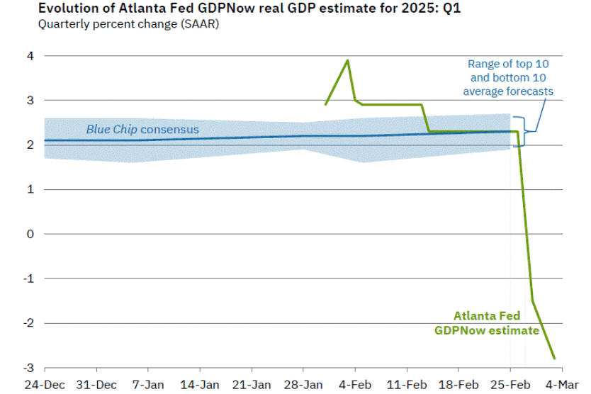
In a post earlier this week, we noted that according to the usually reliable GDPNow forecast from the Federal Reserve Bank of Atlanta, real GDP in the first quarter will decline by 2.8 percent. (The forecast was updated yesterday on the basis of additional data releases to a slightly less pessimistic –2.4 percent decline.) This morning (March 7), the Bureau of Labor Statistics (BLS) released its “Employment Situation” report (often called the “jobs report”) for February. The data in the report show no sign that the U.S. economy is in a recession. We should add the caveat, however, that at the beginning of a recession the data in the jobs report can be subject to large revisions.

The jobs report has two estimates of the change in employment during the month: one estimate from the establishment survey, often referred to as the payroll survey, and one from the household survey. As we discuss in Macroeconomics, Chapter 9, Section 9.1 (Economics, Chapter 19, Section 19.1), many economists and Federal Reserve policymakers believe that employment data from the establishment survey provide a more accurate indicator of the state of the labor market than do either the employment data or the unemployment data from the household survey. (The groups included in the employment estimates from the two surveys are somewhat different, as we discuss in this post.)

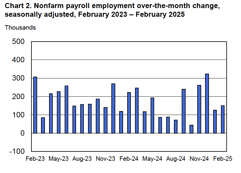
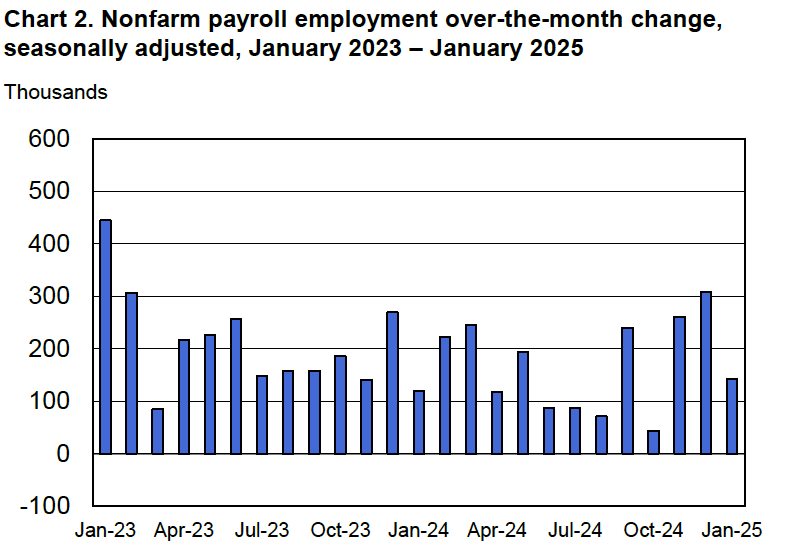
According to the establishment survey, there was a net increase of 151,000 jobs during February. This increase was below the increase of 160,000 that economists had forecast. The previously reported increase for December was revised upward, while the previously reported increase for January was revised downward. The net change in jobs, taking the revisions for those two months together, was 2,000 lower than originally estimated. (The BLS notes that: “Monthly revisions result from additional reports received from businesses and government agencies since the last published estimates and from the recalculation of seasonal factors.”) The following figure from the jobs report shows the net change in payroll employment for each month in the last two years.

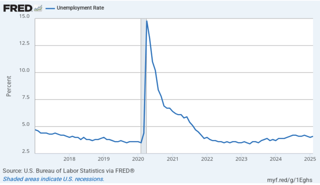
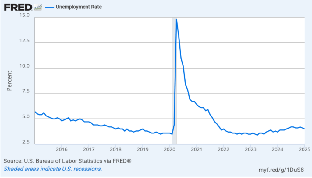
The unemployment rate rose slightly to 4.1 percent in February from 4.0 percent in January. As the following figure shows, the unemployment rate has been remarkably stable in recent months, staying between 4.0 percent and 4.2 percent in each month since May 2024. Last December, the members of the Federal Open Market Committee (FOMC) forecast that the unemployment rate for 2025 would average 4.3 percent.

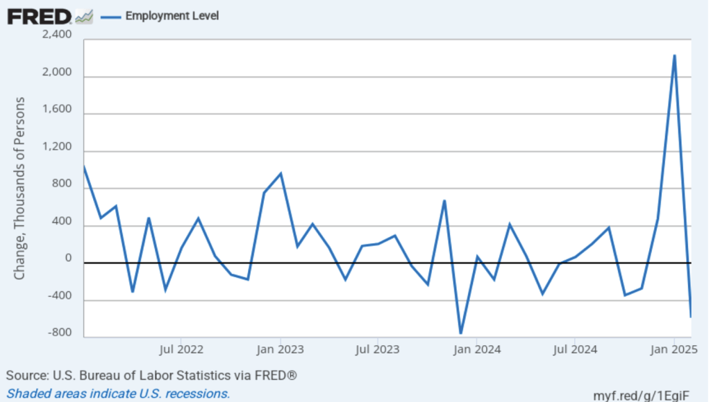
As the following figure shows, the net change in jobs from the household survey moves much more erratically than does the net change in jobs from the establishment survey. The net change in jobs as measured by the household survey for February showed a sharp decrease of 588,000 jobs following a very large increase of 2,234,000 jobs in January. In any particular month, the story told by the two surveys can be inconsistent with employment increasing in one survey while falling in the other. The difference was particularly dramatic this month. (In this blog post, we discuss the differences between the employment estimates in the two surveys.)

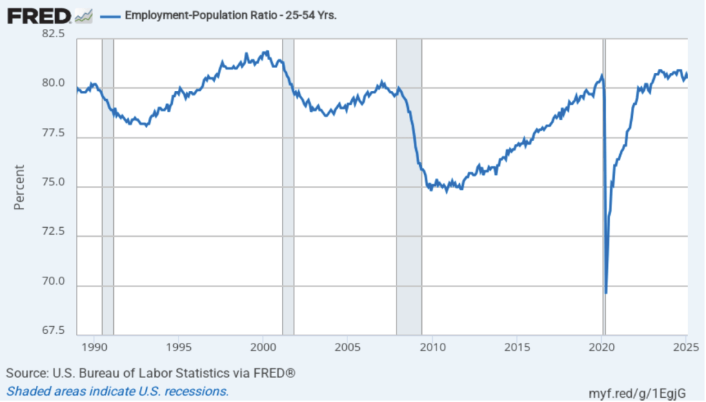
Another concerning sign in the household survey is the fall in the employment-population ratio for prime age workers—those aged 25 to 54. The ratio declined from 80.7 percent in January to 80.5 percent in February. Although the employment-population is still high relative to the average level since 2001, it’s now well below the high of 80.9 percent in mid-2024. Continuing declines in this ratio would indicate a significant softening in the labor market.

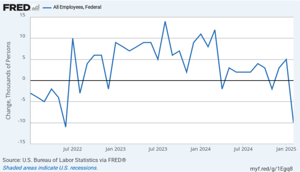
It’s unclear how many federal workers have been laid off since the Trump Administration took office. The household survey shows a decline in total federal government employment of 10,000 in February. The household survey was conducted in the week that included February 12, so, it’s possible that next month’s jobs report may find a more significant decline.

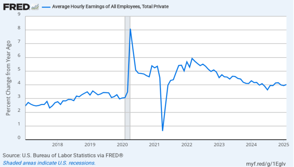
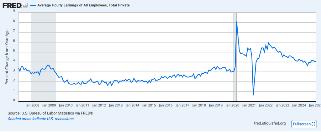
The establishment survey also includes data on average hourly earnings (AHE). As we noted in this post, many economists and policymakers believe the employment cost index (ECI) is a better measure of wage pressures in the economy than is the AHE. The AHE does have the important advantage of being available monthly, whereas the ECI is only available quarterly. The following figure shows the percentage change in the AHE from the same month in the previous year. The AHE increased 4.0 percent in February, up slightly from 3.9 percent in January.

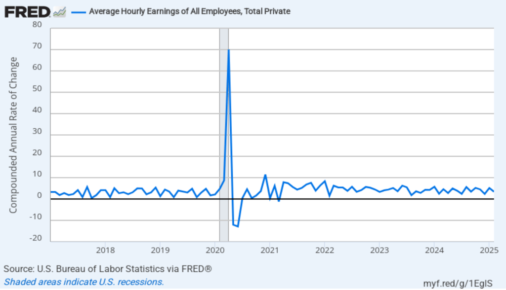
The following figure shows wage inflation calculated by compounding the current month’s rate over an entire year. (The figure above shows what is sometimes called 12-month wage inflation, whereas this figure shows 1-month wage inflation.) One-month wage inflation is much more volatile than 12-month wage inflation—note the very large swings in 1-month wage inflation in April and May 2020 during the business closures caused by the Covid pandemic. The February 1-month rate of wage inflation was 3.4 percent, a decline from the surprisingly high 5.2 percent rate in December. Whether measured as a 12-month increase or as a 1-month increase, AHE is still increasing somewhat more rapidly than is consistent with the Fed achieving its 2 percent target rate of price inflation.

Today’s jobs report leaves the situation facing the Federal Reserve’s policy-making Federal Open Market Committee (FOMC) largely unchanged. There are some indications that the economy may be weakening, as shown by some of the data in the jobs report and by some of the data incorporated by the Atlanta Fed in its pessimistic nowcast of first quarter real GDP. But the Fed hasn’t yet brought inflation down to its 2 percent annual target. In addition, it’s unclear how the Trump Administration’s policies—particularly with respect to tariff increases—might affect the economy. Speaking today at an event at the University of Chicago, Fed Chair Jerome Powell observed the following:

“Looking ahead, the new Administration is in the process of implementing significant policy changes in four distinct areas: trade, immigration, fiscal policy, and regulation. It is the net effect of these policy changes that will matter for the economy and for the path of monetary policy. While there have been recent developments in some of these areas, especially trade policy, uncertainty around the changes and their likely effects remains high. As we parse the incoming information, we are focused on separating the signal from the noise as the outlook evolves. We do not need to be in a hurry, and are well positioned to wait for greater clarity.”

The likeliest outcome is that the FOMC will keep its target for the federal funds rate unchanged, perhaps for several meetings, unless additional data are released that clearly show the economy to be weakening.

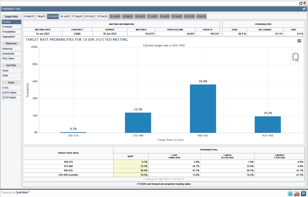
One indication of expectations of future cuts in the target for the federal funds rate comes from investors who buy and sell federal funds futures contracts. (We discuss the futures market for federal funds in this blog post.) The data from the futures market indicates that investors don’t expect that the FOMC will cut its target for the federal funds rate at either its March 18–19 or May 6–7 meetings. As shown in the following figure, only at the FOMC’s June 17–18 meeting do investors assign a greater than 50 percent probability to the committee cutting its target. As of this afternoon, investors assign a probability of only 19.2 percent to the FOMC keeping its target unchanged at 4.25 percent to 4.50 percent at that meeting. They assign a probability of 80.8 percent to the committee cutting its target rate by at least 0.25 percentage point (25 basis points) at that meeting.

Are We in a Recession? Depends on Which Forecast You Believe

Image generated by GTP-4o of people engaging in economic forecasting

How do we know when we’re in a recession? Most economists and policymakers accept the decisions of the National Bureau of Economic Research (NBER), a private research group located in Cambridge, Massachusetts (see Macroeconomics, Chapter 10, Section 10.3). Typically, the NBER is slow in announcing that a recession has begun because it takes time to gather and analyze economic data. The NBER didn’t announce that a recession had begun in December 2007 until 11 months later in November 2008. When the NBER announced in June 2020 that a recession had begun in February 2020, it was considered to be an unusually fast decision.

On its website, the NBER notes that: “The NBER’s traditional definition of a recession is that it is a significant decline in economic activity that is spread across the economy and that lasts more than a few months.” The NBER lists the data it considers when determining whether a recession has begun (or ended), including: “real personal income less transfers (PILT), nonfarm payroll employment, real personal consumption expenditures, manufacturing and trade sales adjusted for price changes, employment as measured by the household survey, and industrial production.” In practice, it is normally the case that an NBER business cycle peak coincides with the peak in nonfarm payroll employment and an NBER business cycle trough coincides with a trough in the same employment series.

Of course, policymakers at the Fed don’t wait until the NBER announces that a recession has begun when formulating monetary policy. Members of the Fed’s policymaking Federal Open Market Committee (FOMC) monitor a wide range of data series as the series become available. The broadest measure of the state of the economy is real GDP, which is only available quarterly, and the data are released with a lag. For instance, the Bureau of Economic Analysis’s “advance” (first) estimate of real GDP in the first quarter of 2025 won’t be released until April 30.

Given the importance of GDP, there are several groups that attempt to nowcast GDP. A nowcast is a forecast that incorporates all the information available on a certain date about the components of spending that are included in GDP. The Federal Reserve Bank of New York and the Federal Reserve Bank of Atlanta both release nowcasts of GDP. They use different methodologies, so their forecasts are not identical. Today (March 3), the two estimates are surprisingly far apart. First, here is the nowcast from the NY Fed:

This nowcast indicates that real GDP will grow in the first quarter of 2025 at a 2.94 percent annual rate. That would be an increase from growth of 2.3 percent in the fourth quarter of 2024.

The nowcast from the Atlanta Fed—which they call GDPNow—is strikingly different:

The Atlanta Fed nowcast indicates that real GDP in the first quarter of 2025 will decline by 2.8 percent at an annual rate. If accurate, this forecast indicates that—far from the solid expansion in economic activity that the NY Fed is forecasting—the U.S. economy in the first quarter of 2025 will contract at the fastest rate since the first quarter of 2009, near the end of the severe 2007–2009 downturn (leaving aside the highly unusual declines in the first three quarters of 2020 during the Covid pandemic).

What explains such a large difference between these two forecasts? First, note that the Atlanta Fed includes in its graphic the range of forecasts from Blue Chip Indicators. These forecasts are collected from 50 or more economists who work in the private sector at banks, brokerages, manufacturers, and other firms. The graphic shows that the Blue Chip forecasters do not expect that the economy grew as much as the NY Fed’s nowcast indicates, but the forecasters do expect solid growth rate of 2 percent or more. So, the Atlanta Fed’s forecast appears to be an outlier.

Second, the NY Fed updates its nowcast only once per week, whereas the Atlanta Fed updates its forecast after the release of each data series that enters its model. So, the NY Fed nowcast was last updated on February 28, while the Atlanta Fed nowcast was updated today. Since February 28, the Atlanta Fed has incorporated into its nowcast data on the Institute for Supply Management (ISM) manufacturing index and data on construction spending from the Census Bureau. Incorporating these data resulted in the Atlanta Fed’s nowcast of first quarter real GDP growth declining from –1.5 percent on February 28 to –2.8 percent on March 3.

But incorporating more data explains only part of the discrepancy between the two forecasts because even as of February 28 the forecasts were far apart. The remaining discrepancy is due to the different methodologies employed by the economists at the two regional Feds in building their nowcasting models.

Which forecast is more accurate? We’ll get some indication on Friday (March 7) when the Bureau of Labor Statistics (BLS) releases its “Employment Situation” report for February. Economists surveyed are expecting that the payroll survey will estimate that there was a net increase of 160,000 jobs in February, up from a net increase of 143,000 jobs in January. If that expectation is accurate, it would seem unlikely that production declined in the first quarter to the extent that the Atlanta Fed nowcast is indicating. But, as we discuss in this blog post from 2022, macro data can be unreliable at the beginning of a recession. If we are currently in a recession, then even an initial estimate of a solid net increase in jobs in February could later be revised sharply downward.

CPI Inflation in January Is Higher than Expected

Image generated by GTP-4o illustrating inflation

On February 12, the Bureau of Labor Statistics (BLS) released its monthly report on the consumer price index (CPI). The following figure compares headline inflation (the blue line) and core inflation (the dotted green line).

  • The headline inflation rate, which is measured by the percentage change in the CPI from the same month in the previous month, was 3.0 percent in January—up from 2.9 percent in December. 
  • The core inflation rate, which excludes the prices of food and energy, was 3.3 percent in January—up from 3.2 percent in December. 

Headline inflation and core inflation were both above what economists surveyed had expected.

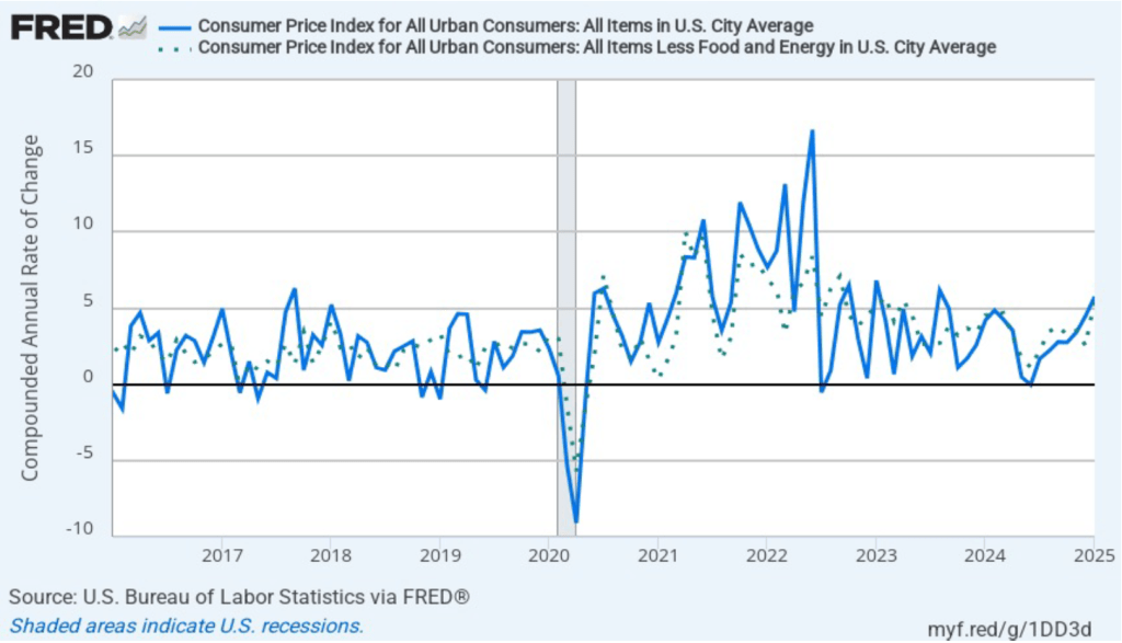
In the following figure, we look at the 1-month inflation rate for headline and core inflation—that is the annual inflation rate calculated by compounding the current month’s rate over an entire year. Calculated as the 1-month inflation rate, headline inflation (the blue line) jumped from 4.5 percent in December to 5.7 percent in January—following a large jump in inflation from November to December. Core inflation (the dotted green line) more than doubled from 2.5 percent in December to 5.5 percent in January.

Overall, considering 1-month and 12-month inflation together, today’s data are concerning. One-month headline inflation is the highest it’s been since August 2023. One-month core inflation is the highest it’s been since April 2023. This month’s CPI report reinforces the conclusion from other recent inflation reports that progress on lowering inflation appears to have stalled. So, the probability of a “no landing” outcome, with inflation remaining above the Fed’s target for an indefinite period, seems to have increased. 

Of course, it’s important not to overinterpret the data from a single month. The figure shows that 1-month inflation is particularly volatile. Also note that the Fed uses the personal consumption expenditures (PCE) price index, rather than the CPI, to evaluate whether it is hitting its 2 percent annual inflation target.

As we’ve discussed in previous blog posts, Federal Reserve Chair Jerome Powell and his colleagues on the Fed’s policymaking Federal Open Market Committee (FOMC) have been closely following inflation in the price of shelter. The price of “shelter” in the CPI, as explained here, includes both rent paid for an apartment or a house and “owners’ equivalent rent of residences (OER),” which is an estimate of what a house (or apartment) would rent for if the owner were renting it out. OER is included in the CPI to account for the value of the services an owner receives from living in an apartment or house.

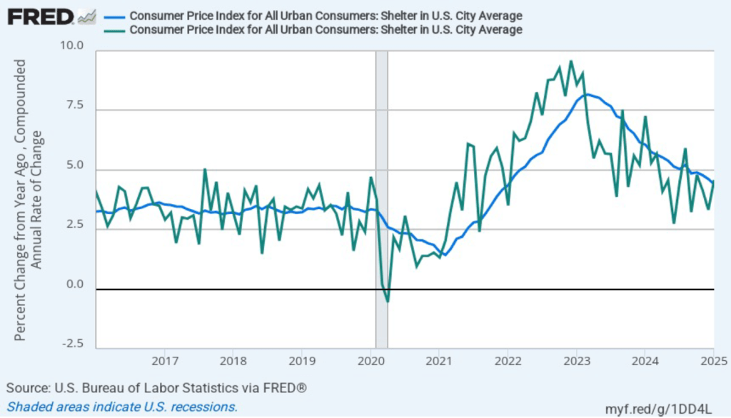
As the following figure shows, inflation in the price of shelter has been a significant contributor to headline inflation. The blue line shows 12-month inflation in shelter, and the green line shows 1-month inflation in shelter. Twelve-month inflation in shelter has been declining since the spring of 2023, but in January it was still relatively high at 4.4 percent. One-month inflation in shelter—which is much more volatile than 12-month inflation in shelter—rose sharply from 3.3 percent in December to 4.6 percent in January. Clearly a worrying sign given that many economists were expecting that shelter inflation would continue to slow.

To better estimate of the underlying trend in inflation, some economists look at median inflation and trimmed mean inflation.

  • Median inflation is calculated by economists at the Federal Reserve Bank of Cleveland and at Ohio State University. If we listed the inflation rate in each individual good or service in the CPI, median inflation is the inflation rate of the good or service that is in the middle of the list—that is, the inflation rate in the price of the good or service that has an equal number of higher and lower inflation rates. 
  • Trimmed-mean inflation drops the 8 percent of goods and services with the highest inflation rates and the 8 percent of goods and services with the lowest inflation rates. 

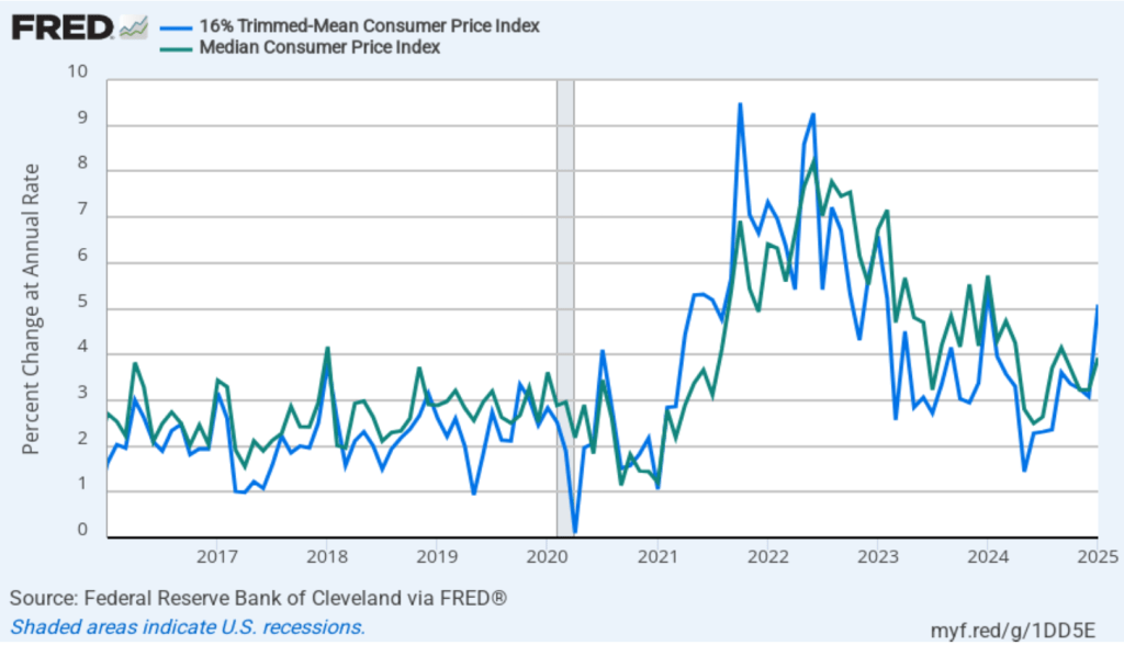
The following figure shows that 12-month trimmed-mean inflation (the blue line) jumped from 3.1 percent in December to 5.2 percent in January. Median inflation (the green line), which had been stable over the past five months, increased from 3.2 percent in December to 3.9 percent in January.

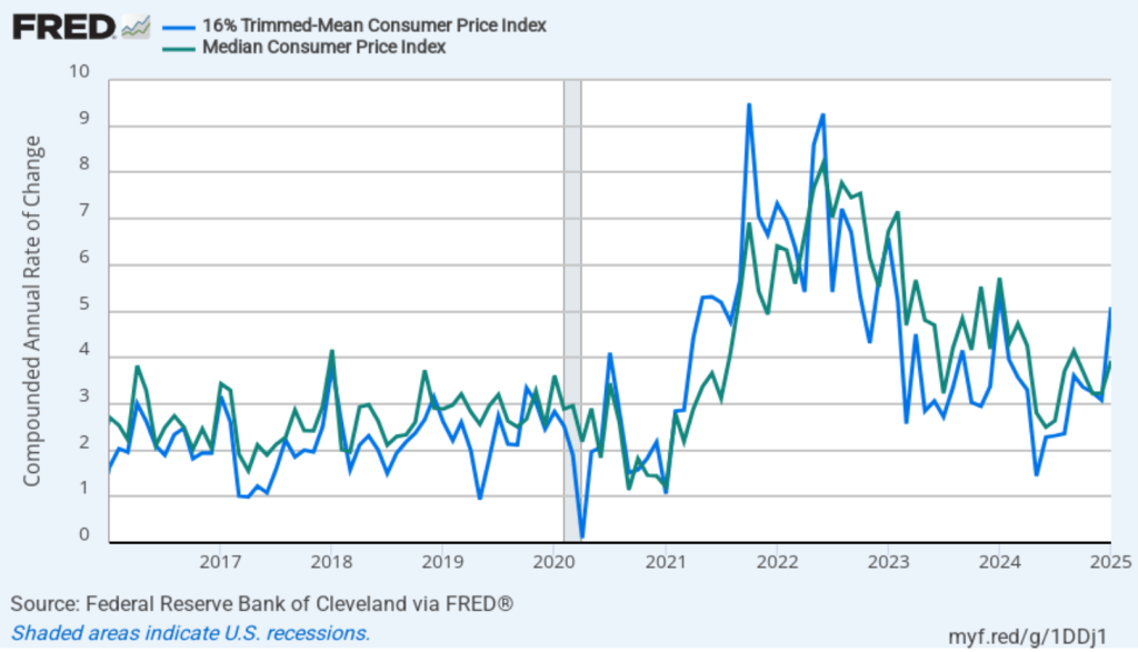
The following figure shows 1-month median and trimmed-mean inflation. One-month trimmed-mean inflation jumped from 3.1 percent in December to 5.1 percent in January. One-month median inflation rose from 3.2 percent in December to 3.9 percent in January. These data provide confirmation that (1) CPI inflation at this point is running higher than a rate that would be consistent with the Fed achieving its inflation target, and (2) that progress toward the target has slowed.

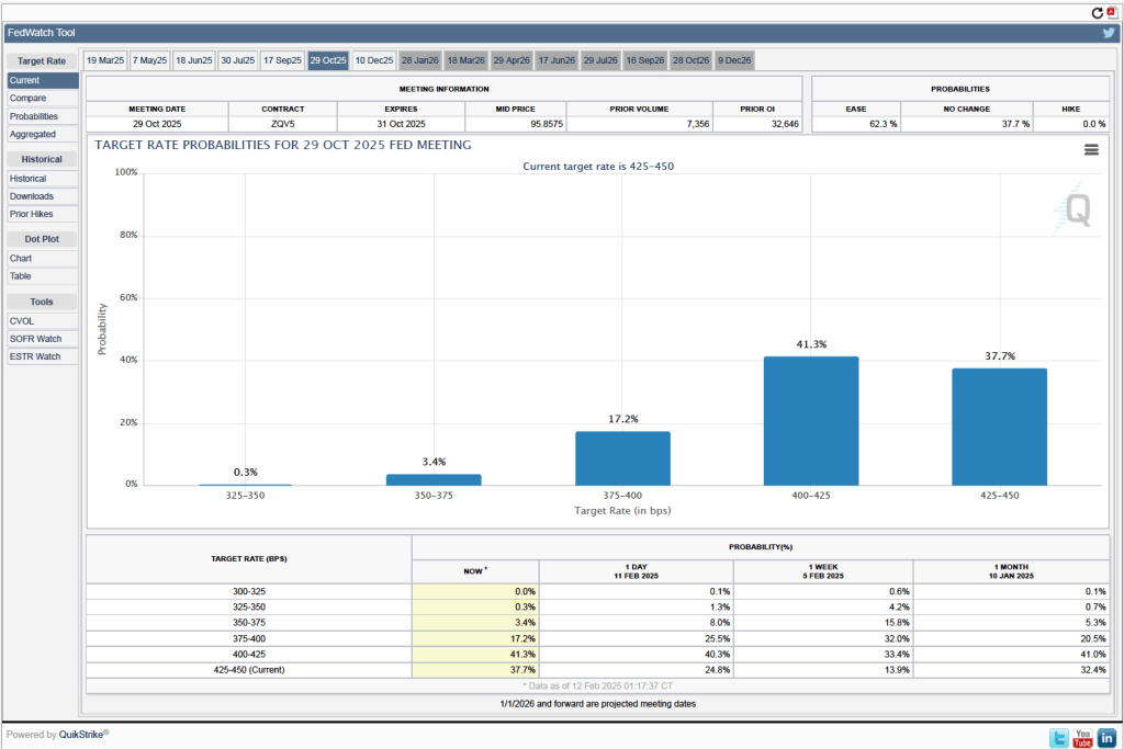
Looking at the futures market for federal funds, investors who buy and sell federal funds futures contracts are not expecting that the Fed’s policymaking Federal Open Market Committee (FOMC) will cut its target for the federal funds until this fall. (We discuss the futures market for federal funds in this blog post.) Investors assign a higher probability to the FOMC leaving its target range for the federal funds rate unchanged at 4.25 percent to 4.50 percent at its January, March, June, July, and September meetings. It’s not until the FOMC’s meeting on October 28-29 that, as shown below, investors assign a higher probability to a rate cut than to the committee leaving the rate unchanged.

The Strikingly Large Role of Foreign-Born Workers in the Growth of the U.S. Labor Force

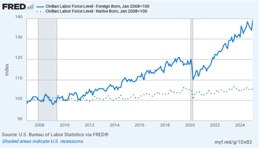
As we noted in a recent post on the latest jobs report, the Bureau of Labor Statistics (BLS) has updated the population estimates in its household employment survey to reflect the revised population estimates from the Census Bureau. The census now estimates that the civilian noninstitutional population was about 2.9 million larger in December 2024 than it had previously estimated. The original undercount was significantly driven by an underestimate of the increase in the immigrant population.

The following figure shows the more rapid growth of foreign-born workers in recent years in comparison with the growth in native-born workers. In the figure, we set the number of native-born workers and the number of foreign-born workers both equal to 100 in January 2007. Between January 2007 and January 2025, the number of foreign-born workers increased by 40 percent, while the number of native-born workers increased by only 6 percent.

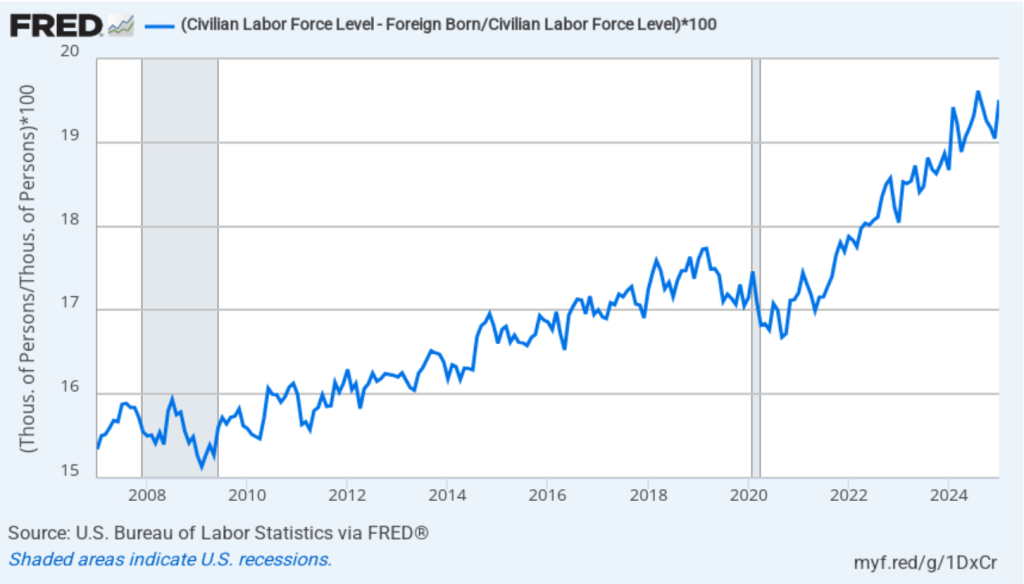
As the following figure shows, although foreign-born workers are an increasingly larger percentage of the total labor force, native-born workers are still a large majority of the labor force. Foreign-born workers were 15.3 percent of the labor force in January 2007 and 19.5 percent of the labor force in January 2025. Foreign-born workers accounted for about 56 percent of the increase in the total labor force over the period from January 2007 to January 2025.

H/T to Jason Furman for pointing us to the BLS data.

Strong Jobs Report in the Context of Annual Revisions to the Establishment and Household Surveys

Photo courtesy of Lena Buonanno

This morning (February 7), the Bureau of Labor Statistics (BLS) released its “Employment Situation” report (often called the “jobs report”) for January. This report was particularly interesting because it includes data reflecting the annual benchmark revision to the establishment, or payroll, survey and the annual revision of the household survey data to match new population estimates from the Census Bureau.

According to the establishment survey, there was a net increase of 143,000 jobs during January. This increase was below the increase of 169,000 to 175,000 that economists had forecast in surveys by the Wall Street Journal and bloomberg.com. The somewhat weak increase in jobs during January was offset by upward revisions to the initial estimates for November and December. The previously reported increases in employment for those months were revised upward by a total of 100,000 jobs. (The BLS notes that: “Monthly revisions result from additional reports received from businesses and government agencies since the last published estimates and from the recalculation of seasonal factors.”)

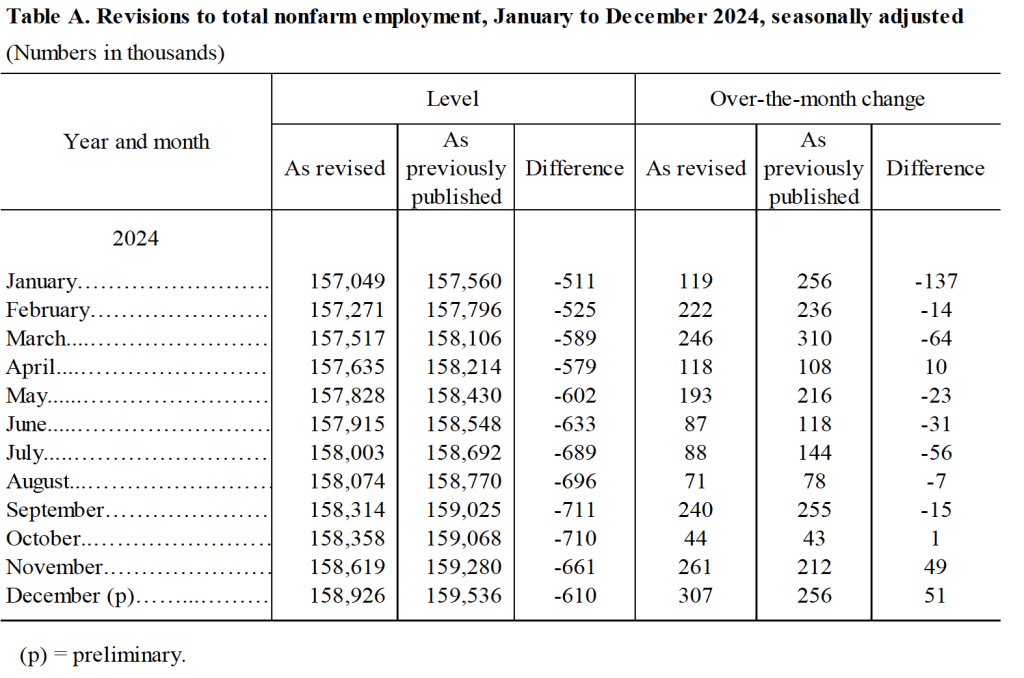
The BLS also announced the results of its annual revision of the payroll employment data benchmarked to March 2024. The revisions are mainly based on data from the Quarterly Census of Employment and Wages (QCEW). The data in payroll survey are derived from a sample of 300,000 establishments, whereas the QCEW is based on a much more comprehensive count of workers covered by state unemployment insurance programs. The revisions indicated that growth in payroll employment between March 2023 and March 2024 had been overstated by 598,000 jobs. Although large in absolute scale, the revisions equal only 0.4 percent of total employment. In addition, as we discussed in this blog post last August, initially the BLS had estimated that the overstatement in employment gains during this period was an even larger 818,000 jobs. (The BLS provides a comprehensive discuss of its revisions to the establishment employment data here.)

The following table shows the revised estimates for each month of 2024, based on the new benchmarking.

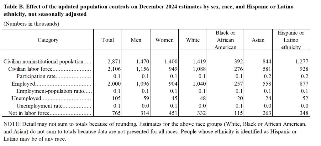
The BLS also revised the household survey data to reflect the latest population estimates from the census bureau. Unlike with the establishment data, the BLS doesn’t adjust the historical household data in light of the population benchmarking. However, the BLS did include two tables in this month’s jobs report illustrating the effect of the new population benchmark. The following table from the report shows the effect of the benchmarking on some labor market data for December 2024. The revision increases the estimate of the civilian noninstitutional population by nearly 3 million, most of which is attributable to an increase in the estimated immigrant population. The increase in the estimate of the number of employed workers was also large at 2 million. (The BLS provides a discussion of the effects of its population benchmarking here.)

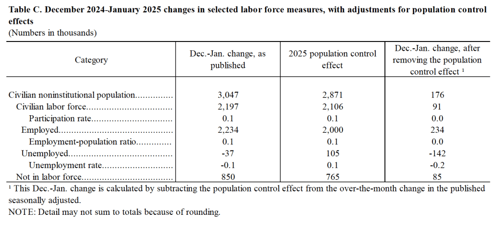
The following table shows how the population benchmarking affects changes in estimates of labor market variables between December 2024 and January 2025. The population benchmarking increases the net number of jobs created in January by 234,000 and reduces the increase in the number of persons unemployed by 142,000.

As the following figure shows, the unemployment rate, as reported in the household survey, decreased from 4.1 percent in December to 4.0 percent in January. The figure shows that the unemployment rate has fluctuated in a fairly narrow range over the past year.

The establishment survey also includes data on average hourly earnings (AHE). As we’ve noted in previous posts, many economists and policymakers believe the employment cost index (ECI) is a better measure of wage pressures in the economy than is the AHE. The AHE does have the important advantage of being available monthly, whereas the ECI is only available quarterly. The following figure shows the percentage change in the AHE from the same month in the previous year. AHE increased 4.1 percent in January, which was unchanged from the December increase. By this measure, wage growth is still somewhat higher than is consistent with annual price inflation running at the Fed’s target of 2 percent.

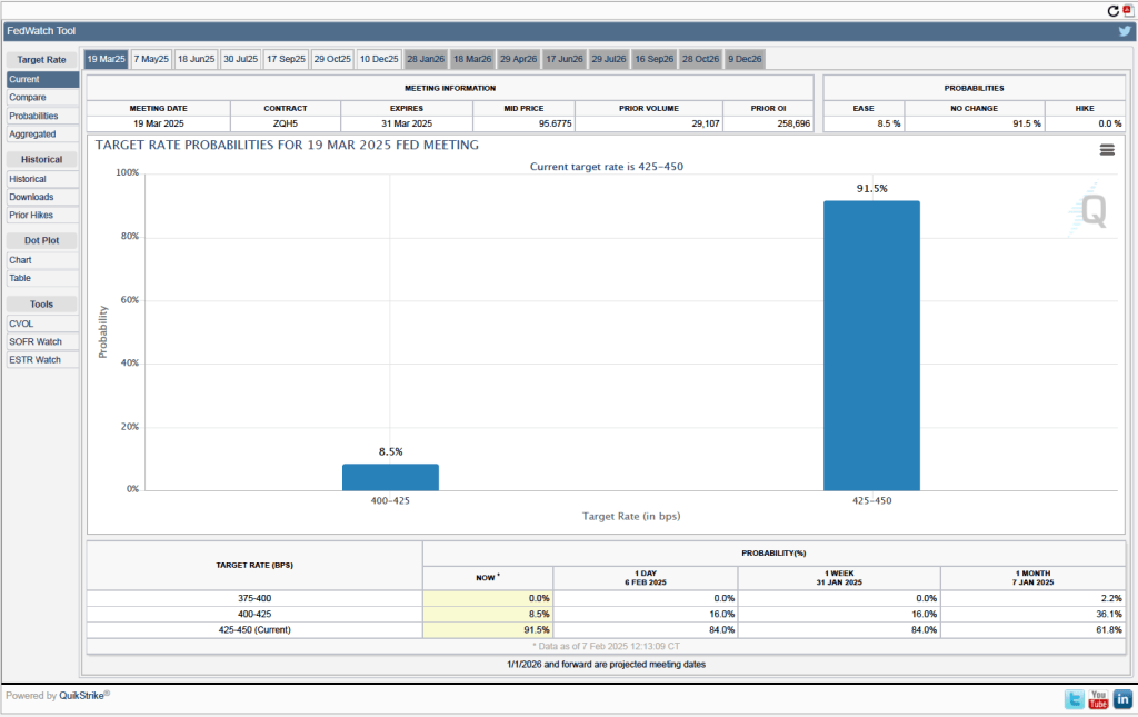
There isn’t much in today’s jobs report to change the consensus view that the Fed’s policymaking Federal Open Market Committee (FOMC) will leave its target for the federal funds rate unchanged at its next meeting on March 18-19. One indication of expectations of future rate cuts comes from investors who buy and sell federal funds futures contracts. (We discuss the futures market for federal funds in this blog post.) As shown in the following figure, today these investors assign a probability of 91.5 percent to the FOMC keeping its target range for the federal funds rate unchanged at the current range of 4.25 percent to 4.50 percent at the March meeting. Investors assign a probability of only 8.5 percent to the FOMC cutting its target range by 25 basis points at that meeting.

JOLTS Report Indicates the Labor Market Remains Strong

Image generated by ChatGTP-4o

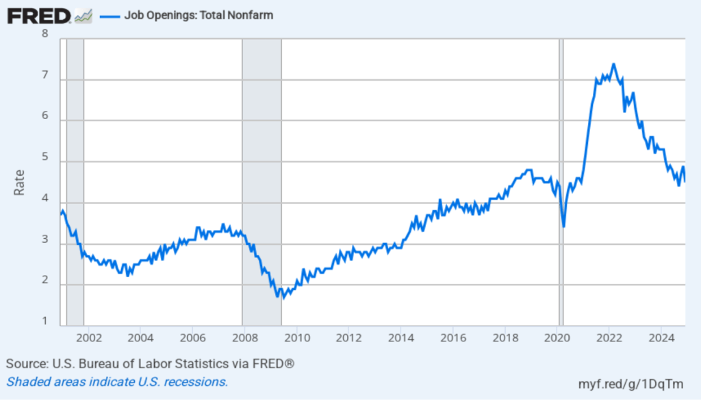
Earlier this week, the Bureau of Labor Statistics (BLS) released its “Job Openings and Labor Turnover” (JOLTS) report for December 2024. The report indicated that labor market conditions remain strong, with most indicators being in line with their values from 2019, immediately before the pandemic. The following figure shows that, at 4.5 percent, the rate of job openings remains in the same range as during the previous six months. While well down from the peak job opening rate of 7.4 percent in March 2022, the rate of job openings was the same as during the summer of 2019 and above the rates during most of the period following the Great Recession of 2007–2009.

(The BLS defines a job opening as a full-time or part-time job that a firm is advertising and that will start within 30 days. The rate of job openings is the number of job openings divided by the number of job openings plus the number employed workers, multiplied by 100.)

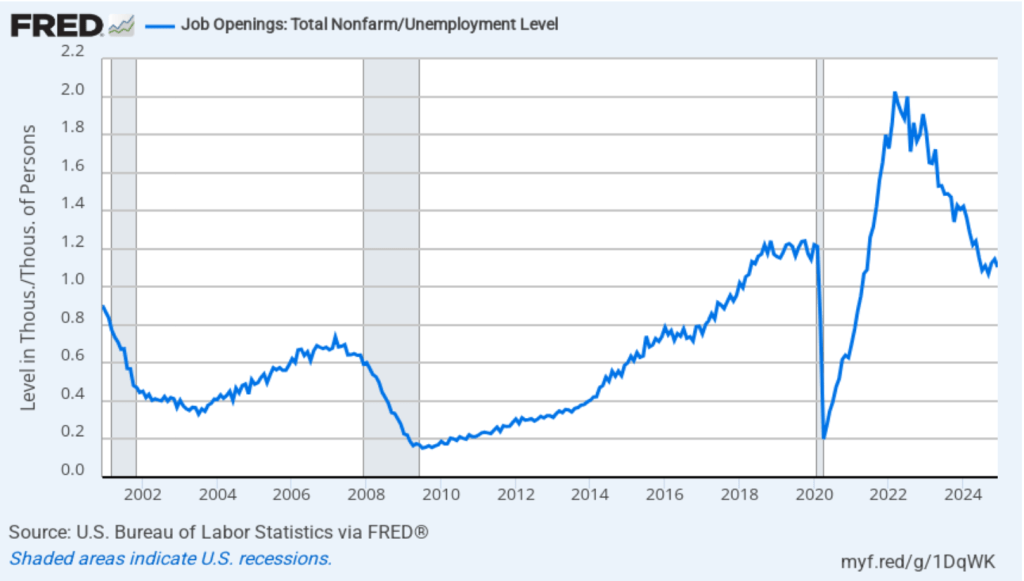
In the following figure, we compare the total number of job openings to the total number of people unemployed. The figure shows a slow decline from a peak of more than 2 job openings per unemployed person in the spring of 2022 to 1.1 job openings per unemployed person in December 2024—about the same as in 2019 and early 2020, before the pandemic. Note that the number is still above 1.0, indicating that the demand for labor is still high, although no higher than during the strong labor market of 2019.

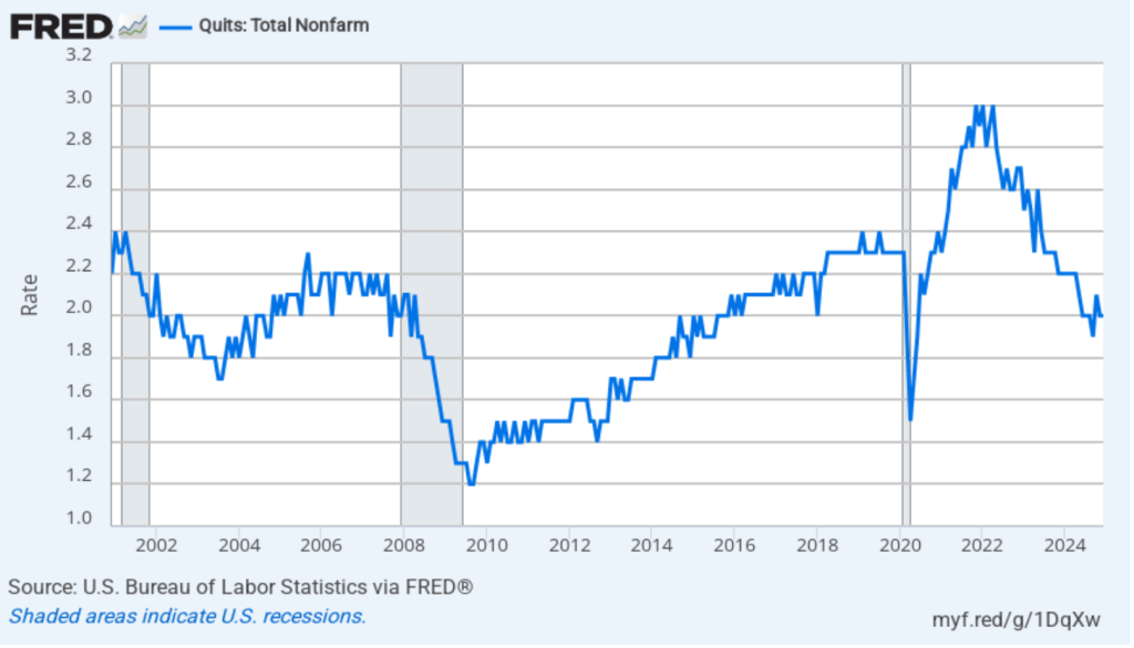
The rate at which workers are willing to quit their jobs is an indication of how they perceive the ease of finding a new job. As the following figure shows, the quit rate declined slowly from a peak of 3 percent in late 2021 and early 2022 to 2.0 percent in July 2024, the same value as in December 2024. That rate is below the rate during 2019 and early 2020. By this measure, workers’ perceptions of the state of the labor market may have deteriorated slightly in recent months.

The JOLTS data indicate that the labor market is about as strong as it was in the months prior to the start of the pandemic, but it’s not as historically tight as it was through most of 2022 and 2023. In recent months, workers may have become less optimistic about finding a new job if they quit their current job. The “Great Quitting,” which was widely discussed in the business press during the period of high quit rates in 2022 and 2023 would seem to be over.

On Friday morning, the BLS will release its “Employment Situation” report for January, which will provide additional data on the state of the labor market. (Note that the data in the JOLTS report lag the data in the “Employment Situation” report by one month.)