Ch25: Monetary Policy – Page 11 – HubbardOBrienEconomics.com Blog

How Should the Fed Interpret the Monthly Employment Reports?

Jerome Powell arriving to testify before Congress. (Photo from Bloomberg News via the Wall Street Journal.)

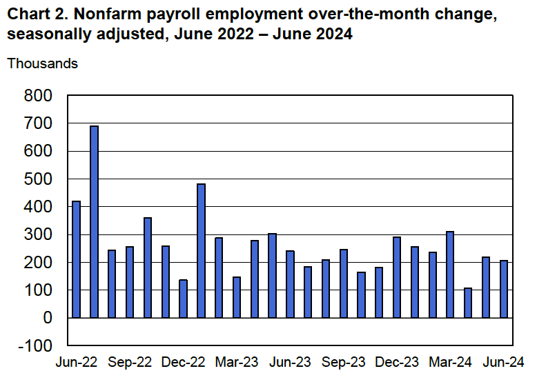
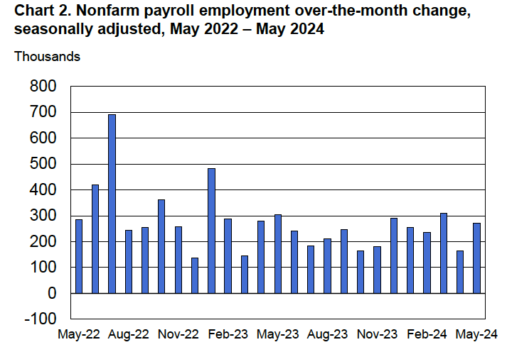
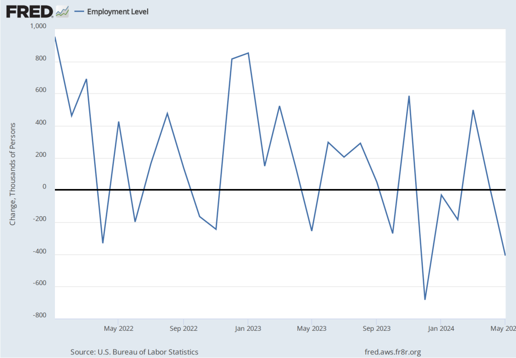
Each month the Bureau of Labor Statistics (BLS) releases its “Employment Situation” report. As we’ve discussed in previous blog posts, discussions of the report in the media, on Wall Street, and among policymakers center on the estimate of the net increase in employment that the BLS calculates from the establishment survey.

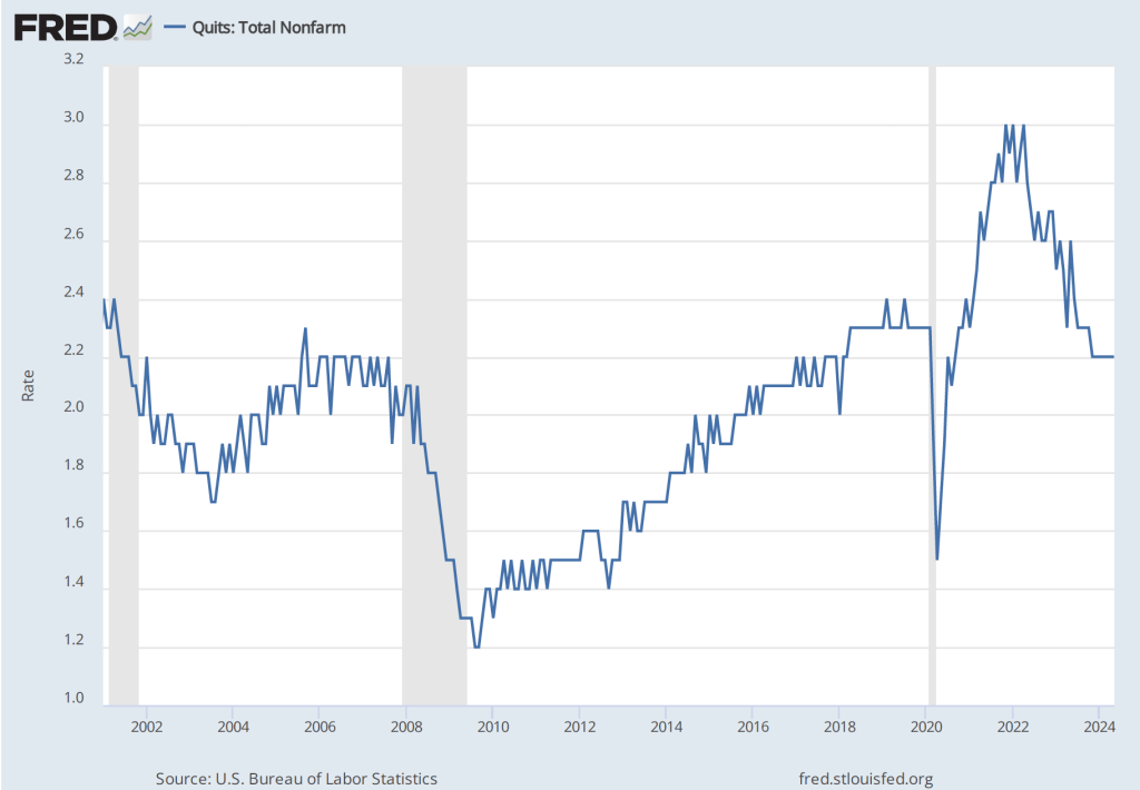
How should the members of the Fed’s policy-making Federal Open Market Committee interpret these data? For instance, the BLS reported that the net increases in employment in June was 206,000. (Always worth bearing in mind that the monthly data are subject to—sometimes substantial—revisions.) Does a net increase of employment of that size indicate that the labor market is still running hot—with the quantity of labor demanded by businesses being greater than the quantity of labor workers are supplying—or that the market is becoming balanced with the quantity of labor demanded roughly equal to the quantity of labor supplied?

On July 9, in testimony before the Senate Banking Committee indicated that his interpretation of labor market data indicate that: “The labor market appears to be fully back in balance.” One interpretation of the labor market being in balance is that the number of net new jobs the economy creates is enough to keep up with population growth. In recent years, that number has been estimated to be 70,000 to 100,000. The number is difficult to estimate with precision for two main reasons:

There is some uncertainty about the number of older workers who will retire. The more workers who retire, the fewer net new jobs the economy needs to create to accommodate population growth.
More importantly, estimates of population growth are uncertain, largely because of disagreements among economists and demographers over the number of immigrants who have entered the United States in recent years.

In calculating the unemployment rate and the size of the labor force, the BLS relies on estimates of population from the Census Bureau. In a January report, the Congressional Budget Office (CBO) argued that the Census Bureau’s estimate of the population of the United States is too low by about 6 million people. As the following figure from the CBO report indicates, the CBO believes that the Census Bureau has underestimated how much immigration has occurred and what the level of immigration is likely to be over the next few years. (In the figure, SSA refers to the Social Security Administration, which also makes forecasts of population growth.)

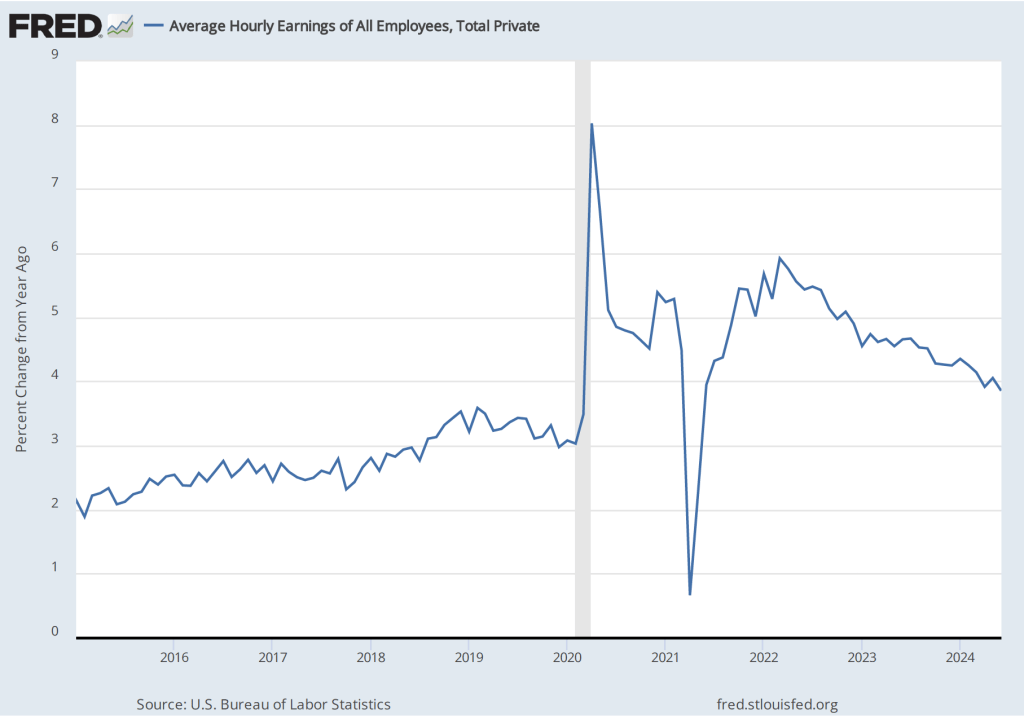
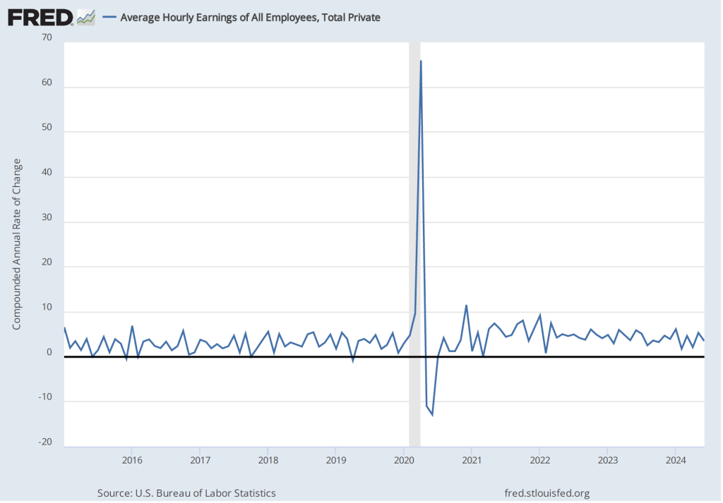
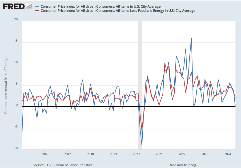
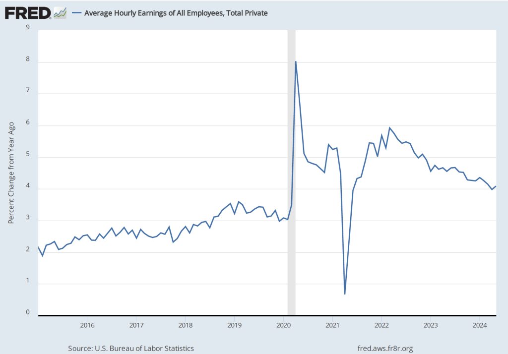
Some economists and policymakers have been surprised that low levels of unemployment and large monthly increases in employment have not resulted in greater upward pressure on wages. If the CBO’s estimates are correct, the supply of labor has been increasing more rapidly than is indicated by census data, which may account for the relative lack of upward pressure on wages. If the CBO’s estimates of population growth are correct, a net increase in employment of 200,000, as occured in June, may be about the number necessary to accommodate growth in the labor force. In other words, Chair Powell would be correct that the labor market was in balance in June.

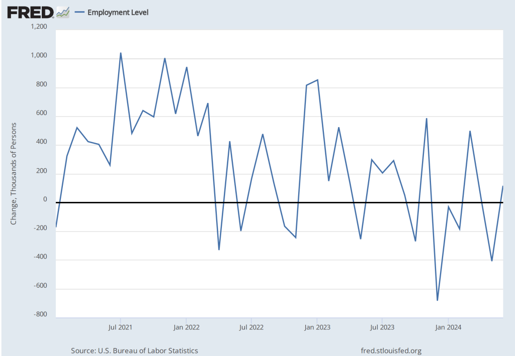
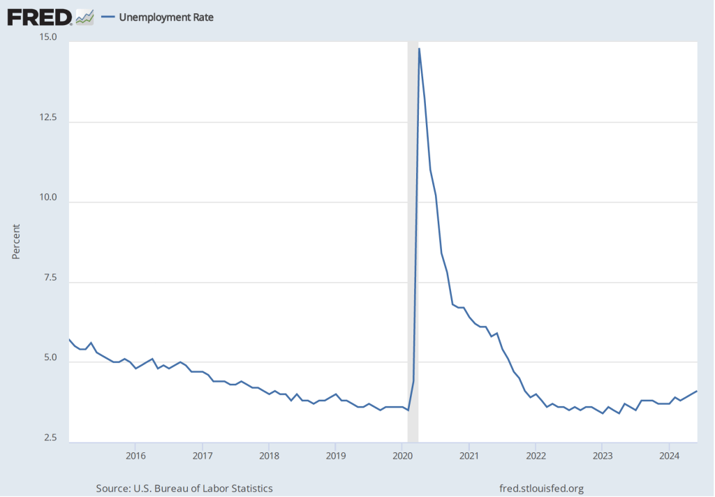
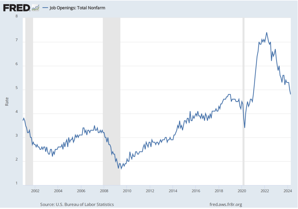
In a recent publication, economists Nicolas Petrosky-Nadeau and Stephanie A. Stewart of the Federal Reserve Bank of San Francisco look at a related concept: breakeven employment growth—the rate of employment growth required to keep the unemployment rate unchanged. They estimate that high rates of immigration during the past few years have raised the rate of breakeven employment growth from 70,000 to 90,000 jobs per month to 230,000 jobs per month. This analysis would be consistent with the fact that as net employment increases have averaged 177,000 over the past three months—somewhat below their estimate of breakeven employment growth—the unemployment rate has increased from 3.8 percent to 4.1 percent.

Latest CPI Report Shows Inflation Continuing to Slow

Image of “a family shopping in a supermarket” generated by ChatGTP 4o.

In testifying before Congress this week, Federal Reserve Chair Jerome Powell indicated that the Fed’s policy-making Federal Open Market Committee (FOMC) was becoming more concerned that it not be too late in reducing its target for the federal funds rate:

“[I]n light of the progress made both in lowering inflation and in cooling the labor market over the past two years, elevated inflation is not the only risk we face. Reducing policy restraint too late or too little could unduly weaken economic activity and employment.”

Powell also noted that: “more good data would strengthen our confidence that inflation is moving sustainably toward 2 percent.” Today (July 11), Powell received more good data as the Bureau of Labor Statistics (BLS) released its monthly report on the consumer price index (CPI), which showed a further slowing in inflation.

As the following figure shows, the inflation rate for June measured by the percentage change in the CPI from the same month in the previous month—headline inflation (the blue line)—was 3.o percent down from 3.3 percent in May. Core inflation (the red line)—which excludes the prices of food and energy—was 3.3 percent in June, down from 3.4 percent in May.

As the following figure shows, if we look at the 1-month inflation rate for headline and core inflation—that is the annual inflation rate calculated by compounding the current month’s rate over an entire year—the declines in the inflation rate are much larger. Headline inflation (the blue line) declined from 0.1 percent in May to –0.7 in June—consumer prices fell during June. Core inflation (the red line) declined from 2.0 percent in May to 0.8 percent in June. Overall, we can say that inflation has cooled further in June, bringing the U.S. economy closer to a soft landing—with the annual inflation rate returning to the Fed’s 2 percent target without the economy being pushed into a recession. (Note, though, that the Fed uses the personal consumption expenditures (PCE) price index, rather than the CPI in evaluating whether it is hitting its 2 percent inflation target.)

The FOMC has been looking closely at inflation in the price of shelter. The price of “shelter” in the CPI, as explained here, includes both rent paid for an apartment or house and “owners’ equivalent rent of residences (OER),” which is an estimate of what a house (or apartment) would rent for if the owner were renting it out. OER is included to account for the value of the services an owner receives from living in an apartment or house.

As the following figure shows, inflation in the price of shelter has been a significant contributor to headline inflation. The blue line shows 12-month inflation in shelter and the red line shows 1-month inflation in shelter. Twelve-month inflation in shelter continued its decline that began in the spring of 2023. One-month inflation in shelter declined substantially from 4.9 percent in May to 2.1 percent in June. These values indicate that the price of shelter may no longer be a significant driver of headline inflation.

Finally, in order to get a better estimate of the underlying trend in inflation, some economists look at median inflation and trimmed mean inflation. Meadin inflation is calculated by economists at the Federal Reserve Bank of Cleveland and Ohio State University. If we listed the inflation rate in each individual good or service in the CPI, median inflation is the inflation rate of the good or service that is in the middle of the list—that is, the inflation rate in the price of the good or service that has an equal number of higher and lower inflation rates. Trimmed mean inflation drops the 8 percent of good and services with the higherst inflation rates and the 8 percent of goods and services with the lowest inflation rates.

As the following figure (from the Federal Reserve Bank of Cleveland) shows, both median inflation (the brown line) and trimmed mean inflation (the blue line) were somewhat higher than either headline CPI inflation or core CPI inflation. One conclusion from these data is that headline and core inflation may be somewhat understating the underlying rate of inflation.

Financial markets are interpreting the most inflation and employment data as indicating that at its meeting on Septembe 17-18 the FOMC is likely to cut its target range for the federal funds rate from the current 5.25 percent to 5.50 to 5.00 percent to 5.25 percent.

Futures markets allow investors to buy and sell futures contracts on commodities–such as wheat and oil–and on financial assets. Investors can use futures contracts both to hedge against risk—such as a sudden increase in oil prices or in interest rates—and to speculate by, in effect, betting on whether the price of a commodity or financial asset is likely to rise or fall. (We discuss the mechanics of futures markets in Chapter 7, Section 7.3 of Money, Banking, and the Financial System.) The CME Group was formed from several futures markets, including the Chicago Mercantile Exchange, and allows investors to trade federal funds futures contracts. The data that result from trading on the CME indicate what investors in financial markets expect future values of the federal funds rate to be. The following chart from the CME’s FedWatch Tool shows the current values from trading of federal funds futures.

The probabilities in the chart reflect investors’ predictions of what the FOMC’s target for the federal funds rate will be after the committee’s September meeting. The chart indicates that investors assign a probability of only 8.1 percent to the FOMC leaving its federal funds rate target unchanged at its September meeting, but a 84.6 percent probability of the committee cutting its target by 0.25 percentage point (and a 7.3 percent probability of the committee cutting its target by 0.50 percent age point).

Latest Jobs Report May Indicate the Labor Market Is Weakening

Image generated by ChatGTP 4o.

Recent macroeconomic data have been sending mixed signals about the state of the U.S. economy. The growth in real GDP, industrial production, retail sales, and real consumption spending has been slowing. Growth in employment has been a bright spot—showing steady net increases in job growth above the level necessary to keep up with population growth. Even here, though, as we discuss in a recent blog post, the data may be overstating the actual strength of the labor market.

This morning (July 5), the Bureau of Labor Statistics (BLS) released its “Employment Situation” report (often referred to as the “jobs report”) for June, which, while seemingly indicating continued strong job growth, also provides some indications that the labor market may be weakening. The jobs report has two estimates of the change in employment during the month: one estimate from the establishment survey, often referred to as the payroll survey, and one from the household survey. As we discuss in Macroeconomics, Chapter 9, Section 9.1 (Economics, Chapter 19, Section 19.1), many economists and policymakers at the Federal Reserve believe that employment data from the establishment survey provides a more accurate indicator of the state of the labor market than do either the employment data or the unemployment data from the household survey. (The groups included in the employment estimates from the two surveys are somewhat different, as we discuss in this post.)

According to the establishment survey, there was a net increase of 206,000 jobs during April. This increase was a little above the increase of 1900,000 to 200,000 that economists had forecast in surveys by the Wall Street Journal and bloomberg.com. The following figure, taken from the BLS report, shows the monthly net changes in employment for each month during the past to years.

It’s notable that the previously reported increases in employment for April and May were revised downward by 110,000 jobs, or by about 25 percent. (The BLS notes that: “Monthly revisions result from additional reports received from businesses and government agencies since the last published estimates and from the recalculation of seasonal factors.”) As we’ve discussed in previous posts (most recently here), revisions to the payroll employment estimates can be particularly large at the beginning of a recession.

As the following figure shows, the net change in jobs from the household survey moves much more erratically than does the net change in jobs in the establishment survey. The net increase in jobs as measured by the household survey increased from –408,000 in May (that is, employment by this measure fell during May) to 116,000 in June.

Note that the BLS also reports a survey for household employment adjusted to conform to the concepts and definitions used to construct the payroll employment series. After this adjustment, over the past 12 months household employment has increased by 32.5 million less than has payroll employment. Clearly, this is a very large discrepancy and may be indicating that the payroll survey is substantially overstating growth in employment.

The unemployment rate, which is also reported in the household survey, ticked up slightly from 4.0 percent to 4.1 percent. Although still low by historical standards, June was the fourth consecutive month in which the unemployment rate increased.

The establishment survey also includes data on average hourly earnings (AHE). As we note in this post, many economists and policymakers believe the employment cost index (ECI) is a better measure of wage pressures in the economy than is the AHE. The AHE does have the important advantage that it is available monthly, whereas the ECI is only available quarterly. The following figure show the percentage change in the AHE from the same month in the previous year. The 3.9 percent increase for June continues a downward trend that began in January and is the smallest increase since June 2021.

The 1-month rate of wage inflation of 3.5 percent in June is a significant decrease from the 5.3 percent rate in May, although it’s unclear whether the decline was an additional sign that the labor market is weakening or reflected the greater volatility in wage inflation when calculated this way.

What effect is today’s job reports likely to have on the Fed’s policy-making Federal Open Market Committee as it considers changes in its target for the federal funds rate? As always, it’s a good idea not to rely too heavily on a single data point—particularly because, as we noted earlier, the establishment survey employment data is subject to substantial revisions. But the Wall Street Journal’s headline that the “Case for September Rate Cut Builds After Slower Jobs Data,” seems likely to be accurate.

Latest JOLTS Report Confirms that the Labor Market Is Returning to Pre-Pandemic Conditions

When inflation began to accelerate in the spring of 2022, the highly unusual situation in the U.S. labor market was one of the reasons. This morning (July 2), the Bureau of Labor Statistics (BLS) released its “Job Openings and Labor Turnover” (JOLTS) report for May 2024. The report proivided more data indicating that the U.S. labor market is continuing its return to pre-pandemic conditions.

The following figures shows the total number of job openings. The BLS defines a job opening as a full-time or part-time job that a firm is advertising and that will start within 30 days. Although the total number of job openings, at 8.1 million, is still somewhat above pre-pandemic levels, it has been gradually declining since reaching a peak of 12.2 million in March 2022.

The next figure shows that, at 4.9 percent, the rate of job openings has continued its slow decline from 7.4 percent in March 2022. The rate in May was just slightly above the rate in January 2019, although it was till above the rates during most of 2019 and early 2020, as well as the rates during most of the period following the Great Recession of 2007–2009. The rate of job openings is defined by the BLS as the number of job openings divided by the number of job openings plus the number of employed workers, multiplied by 100.

In the following figure, we compare the total number of job openings to the total number of people unemployed. The figure shows a slow decline from a peak of more than 2 job openings per unemployed person in the spring of 2022 to 1.2 job openings per employed person in May 2024—the same as in April and about the same as in 2019 and early 2020, before the pandemic. Note that the number is still above 1.0, indicating that the demand for labor is still high, although no higher than during the strong labor market of 2019.

The rate at which workers are willing to quit their jobs is an indication of how they perceive the ease of finding a new job. As the following figure shows, the quit rate declined slowly from a peak of 3 percent in late 2021 and early 2022 to 2.2 percent in November 2023, where it has remained through May 2024. That rate is slightly below the rate during 2019 and early 2020. By this measure, workers perceptions of the state of the labor market seem largely unchanged in recent months.

The JOLTS data indicate that the labor market is about as strong as it was in the months priod to the start of the pandemic, but it’s not as historically tight as it was through most of 2022 and 2023. Speaking today at a conference hosted by the European Central Bank, Fed Chair Jerome Powell was quoted as saying that the Fed had made “a lot of progress” in reducing inflation and that the labor market had made “a pretty substantial” move toward a better balance between labor demand and labor supply.

On Friday morning, the BLS will release its “Employment Situation” report for June, which will provide additional data on the state of the labor market. (Note that the data in the JOLTS report lag the data in the “Employment Situation” report by one month.)

Latest PCE Report Shows Inflation Slowing

Chair Jerome Powell and other members of the Federal Open Market Committee (Photo from federalreserve.gov)

On Friday, June 28, the Bureau of Economic Analysis (BEA) released its “Personal Income and Outlays” report for April, which includes monthly data on the personal consumption expenditures (PCE) price index. Inflation as measured by annual changes in the consumer price index (CPI) receives the most attention in the media, but the Federal Reserve looks instead to inflation as measured by annual changes in the PCE price index to evaluate whether it’s meeting its 2 percent annual inflation target.

The following figure shows PCE inflation (blue line) and core PCE inflation (red line)—which excludes energy and food prices—for the period since January 2015 with inflation measured as the change in the PCE from the same month in the previous year. Measured this way, in May PCE inflation (the blue line) was 2.6 percent in May, down slightly from PCE inflation of 2.7 percent in April. Core PCE inflation (the red line) in May was also 2.6 percent, down from 2.8 percent in April.

The following figure shows PCE inflation and core PCE inflation calculated by compounding the current month’s rate over an entire year. (The figure above shows what is sometimes called 12-month inflation, while this figure shows 1-month inflation.) Measured this way, PCE inflation sharply declined from 3.2 percent in April to -0.1 percent in in May—meaning that consumer prices actually fell during May. Core PCE inflation declined from 3.2 percent in April to 1.0 percent in May. This decline indicates that inflation by either meansure slowed substantially in May, but data for a single month should be interpreted with caution.

The following figure shows another way of gauging inflation by including the 12-month inflation rate in the PCE (the same as shown in the figure above—although note that PCE inflation is now the red line rather than the blue line), inflation as measured using only the prices of the services included in the PCE (the green line), and the trimmed mean rate of PCE inflation (the blue line). Fed Chair Jerome Powell and other members of the Federal Open Market Committee (FOMC) have said that they are concerned by the persistence of elevated rates of inflation in services. The trimmed mean measure is compiled by economists at the Federal Reserve Bank of Dallas by dropping from the PCE the goods and services that have the highest and lowest rates of inflation. It can be thought of as another way of looking at core inflation by excluding the prices of goods and services that had particularly high or particularly low rates of inflation during the month.

Inflation using the trimmed mean measure was 2.8 percent in May (calculated as a 12-month inflation rate), down only slightly from 2.9 percent in April—and still well above the Fed’s target inflation rate of 2 percent. Inflation in services remained high in May at 3.9 percent, down only slightly from 4.0 percent in April.

This month’s PCE inflation data indicate that the inflation rate is still declining towards the Fed’s target, with the low 1-month inflation rates being particularly encouraging. But the FOMC will likely need additional data before deciding to lower the committee’s target for the federal funds rate, which is currently 5.25 percent to 5.50 percent. The next meeting of the FOMC is July 30-31. What do financial markets think the FOMC will decide at that meeting?

The probabilities in the chart reflect investors’ predictions of what the FOMC’s target for the federal funds rate will be after the committee’s July meeting. The chart indicates that investors assign a probability of only 10.3 percent to the FOMC cutting its federal funds rate target by 0.25 percentage point at that meeting and an 89.7 percent probability of the commitee leaving the target unchanged.

In contrast, the following figure shows that investors expect that the FOMC will cut its federal funds rate at the meeting scheduled for September 17-18. Investors assign a 57.9 percent probability of a 0.25 percentage point cut and a 6.2 percent probability of a 0.50 percentage point cut. The committee deciding to leave the target unchanged at 5.25 percent to 5.50 percent is assigned a probability of only 35.9 percent.

Latest CPI Report Shows Slowing Inflation and the FOMC Appears Likely to Cut Its Target for the Federal Funds Rate at Least Once This Year

Image of “a woman shopping in a grocery store” generated by ChatGTP 4o.

Today (June 12) we had the unusual coincidence of the Bureau of Labor Statistics (BLS) releasing its monthly report on the consumer price index (CPI) on the same day that the Federal Open Market Committee (FOMC) concluded a meeting. The CPI report showed that the inflation rate had slowed more than expected. As the following figure shows, the inflation rate for May measured by the percentage change in the CPI from the same month in the previous month—headline inflation (the blue line)—was 3.3 percent—slightly below the 3.4 percent rate that economists surveyed by the Wall Street Journal had expected, and slightly lower than the 3.4 percent rate in April. Core inflation (the red line(—which excludes the prices of food and energy—was 3.4 percent in May, down from 3.6 percent in April and slightly lower than the 3.5 percent rate that economists had been expecting.

As the following figure shows, if we look at the 1-month inflation rate for headline and core inflation—that is the annual inflation rate calculated by compounding the current month’s rate over an entire year—the declines in the inflation rate are much larger. Headline inflation (the blue line) declined from 3.8 percent in April to 0.1 percent in May. Core inflation (the red line) declined from 3.6 percent in April to 2.0 percent in May. Overall, we can say that inflation has cooled in May and if inflation were to continue at the 1-month rate, the Fed will have succeeded in bringing the U.S. economy in for a soft landing—with the annual inflation rate returning to the Fed’s 2 percent target without the economy being pushed into a recession.

But two important notes of caution:

1. It’s hazardous to rely to heavily on data from a single month. Over the past year, the BLS has reported monthly inflation rates that were higher than economists expected and rates that was lower than economists expected. The current low inflation rate would have to persist over at least a few more months before we can safely conclude that the Fed has achieved a safe landing.

2. As we discuss in Macroeconomics, Chapter 15, Section 15.5 (Economics, Chapter 25, Section 25.5), the Fed uses the personal consumption expenditures (PCE) price index, rather than the CPI in evaluating whether it is hitting its 2 percent inflation target. So, today’s encouraging CPI data would have to carry over to the PCE data that the Bureau of Economic Analysis (BEA) will release on January 28 before we can conclude that inflation as the Fed tracks it did in fact slow significantly in April.

The BLS released the CPI report at 8:30 am eastern time. The FOMC began its meeting later in the day and so committee members were able to include in their deliberations today’s CPI data along with other previously available information on the state of the economy. At the close of the meeting, , the FOMC released a statement in which it stated, as expected, that it would leave its target range for the federal funds rate unchanged at 5.25 percent to 5.50 percent. After the meeting, the committee also released—as it typically does at its March, June, September, and December meetings—a “Summary of Economic Projections” (SEP), which presents median values of the committee members’ forecasts of key economic variables. The values are summarized in the following table, reproduced from the release.

The table shows that compared with their projections in March—the last time the FOMC published the SEP—committee members were expecting higher headline and core PCE inflation and a higher federal funds rate at the end of this year. In the long run, committee members were expecting a somewhat highr unemployment rate and somewhat higher federal funds rate than they had expected in March.

Note, as we discuss in Macreconomics, Chapter 14, Section 14.4 (Economics, Chapter 24, Section 24.4 and Essentials of Economics, Chapter 16, Section 16.4), there are twelve voting members of the FOMC: the seven members of the Board of Governors, the president of the Federal Reserve Bank of New York, and presidents of four of the other 11 Federal Reserve Banks, who serve one-year rotating terms. In 2024, the presidents of the Richmond, Atlanta, San Francisco, and Cleveland Feds are voting members. The other Federal Reserve Bank presidents serve as non-voting members, who participate in committee discussions and whose economic projections are included in the SEP.

Prior to the meeting there was much discussion in the business press and among investment analysts about the dot plot, shown below. Each dot in the plot represents the projection of an individual committee member. (The committee doesn’t disclose which member is associated with which dot.) Note that there are 19 dots, representing the 7 members of the Fed’s Board of Governors and all 12 presidents of the Fed’s district banks.

The plots on the far left of the figure represent the projections of each of the 19 members of the value of the federal funds rate at the end of 2024. Four members expect that the target for the federal funds rate will be unchanged at the end of the year. Seven members expect that the committee will cut the target range once, by 0.25 percentage point, by the end of the year. And eight members expect that the cut target range twice, by a total of 0.50 percent point, by the end of the year. Members of the business media and financial analysts were expecting tht the dot plot would project either one or two target rate cuts by the end of the year. The committee was closely divided among those two projections, with the median projection being for a single rate cut.

In its statement following the meeting, the committee noted that:

“In considering any adjustments to the target range for the federal funds rate, the Committee will carefully assess incoming data, the evolving outlook, and the balance of risks. The Committee does not expect it will be appropriate to reduce the target range until it has gained greater confidence that inflation is moving sustainably toward 2 percent. In addition, the Committee will continue reducing its holdings of Treasury securities and agency debt and agency mortgage‐backed securities. The Committee is strongly committed to returning inflation to its 2 percent objective.”

In his press conference after the meeting, Fed Chair Jerome Powell noted that the morning’s CPI report was a “Better inflation report than nearly anyone expected.” But, Powell also noted that: “You don’t want to be motivated any one data point.” Reinforcing the view quoted above in the committee’s statement, Powell emphasized that before cutting the target for the federal funds rate, the committee would need “Greater confidence that inflation is moving back to 2% on a sustainable basis.”

In summary, today’s CPI report was an indication that the Fed is on track to bring about a soft landing, but the FOMC will be closely analyzing macroeconomic data over at least the next few months before it is willing to cut its target for the federal funds rate.

What Does the Latest Jobs Report Tell Us about the State of the U.S. Economy?

Image of “people working in a store” generated by ChatGTP 4o.

This morning (June 7), the Bureau of Labor Statistics (BLS) released its “Employment Situation” report for May. Recent government releases of macroeconomic data have indicated that the expansion of the U.S. economy is slowing. For instance, as we noted in this recent post on the JOLTS report, the labor market seems to be normalizing. Real personal consumption expenditures declined from March to April. The Federal Reserve Bank of New York’s Nowcast of real GDP growth during the current quarter declined from 2.74 percent at the end of April to 1.76 percent at the end of May. That decline reflects some weakness in the data series the economists at the New York Fed use to forecast current real GDP growth

In that context, today’s jobs report was, on balance, surprisingly strong. The report has two estimates of the change in employment during the month: one estimate from the establishment survey, often referred to as the payroll survey, and one from the household survey. As we discuss in Macroeconomics, Chapter 9, Section 9.1 (Economics, Chapter 19, Section 19.1), many economists and policymakers at the Federal Reserve believe that employment data from the establishment survey provides a more accurate indicator of the state of the labor market than do either the employment data or the unemployment data from the household survey. (The groups included in the employment estimates from the two surveys are somewhat different, as we discuss in this post.)

According to the establishment survey, there was a net increase of 272,000 jobs during May. This increase was well below the increase of 190,000 that economists had forecast in a survey by the Wall Street Journal and well above the net increase of 165,000 during April. (Bloomberg’s survey of economists yielded a similar forecast of an increase of 180,000.) The increase was also higher than the 232,000 average monthly increase during the past year. The following figure, taken from the BLS report, shows the monthly net changes in employment for each month during the past two years.

The surprising strength in employment growth in establishment survey was not echoed in the household survey, which reported a net decrease of 408,000 jobs. As the following figure shows, the net change in jobs from the household survey moves much more erratically than does the net change in jobs in the establishment survey, and—as noted earlier—the two surveys are of somewhat different groups. Still, the discrepancy between the two survey was notable.

The unemployment rate, which is also reported in the household survey, ticked up slightly from 3.9 percent to 4.0 percent. This is the first time that the unemployment has reached 4.0 percent since January 2022.

The establishment survey also includes data on average hourly earnings (AHE). As we note in this post, many economists and policymakers believe the employment cost index (ECI) is a better measure of wage pressures in the economy than is the AHE. The AHE does have the important advantage that it is available monthly, whereas the ECI is only available quarterly. The following figure show the percentage change in the AHE from the same month in the previous year. The 4.1 percent increase in May was a slight increase from the 4.0 percent increase in April. The increase in the rate of wage inflation is in contrast with the decline in employment and increase in the unemployment rate in the same report.

The following figure shows wage inflation calculated by compounding the current month’s rate over an entire year. (The figure above shows what is sometimes called 12-month wage inflation, whereas this figure shows 1-month wage inflation.) One-month wage inflation is much more volatile than 12-month inflation—note the very large swings in 1-month wage inflation in April and May 2020 during the business closures caused by the Covid pandemic.
The 1-month rate of wage inflation of 4.9 percent in May is a sharp increase from the 2.8 percent rate in April, although it’s unclear whether the increase represents a significant acceleration in wage inflation or is just reflecting the greater volatility in wage inflation when calculated this way.

To answer the question posed in the title to this post, the latest jobs report is a mixed bag that doesn’t send a clear message as to the state of the economy. The strong increase in employment and the increase in the rate of wage growth indicate that economy may not be slowing sufficiently to result in inflation declining to the Federal Reserve’s 2 percent annual target. On the other hand, the decline in employment as measured in the household survey and the tick up in the unemployment rate, along with the data in the recent JOLTS report, indicate that the labor market may be returning to more normal conditions.

It seems unlikely that this jobs report will have much effect on the thinking of the Fed’s policy-making Federal Open Market Committee (FOMC), which has its next meeting next week on June 11-12.

JOLTS Report Indicates Further Normalizing of the Job Market

Image of “a small business with a help wanted sign in the window” generated by ChatGTP 4o.

This morning (June 4), the Bureau of Labor Statistics (BLS) released its “Job Openings and Labor Turnover” (JOLTS) report for April 2024. The report proivided more data indicating that the U.S. labor market is continuing its return to pre-pandemic conditions. The following figure shows that, at 4.8 percent, the rate of job openings has continued its slow decline from the rate of 7.4 percent in March 2022. The rate in April was the same as the rate in January 2019, although it was till above the rates during most of 2019 and early 2020, as well as the rates during most of the period following the Great Recession of 2007–2009.

The BLS defines a job opening as a full-time or part-time job that a firm is advertising and that will start within 30 days. The rate of job openings is the number of job openings divided by the number of job openings plus the number of employed workers, multiplied by 100.

In the following figure, we compare the total number of job openings to the total number of people unemployed. The figure shows a slow decline from a peak of more than 2 job openings per unemployed person in the spring of 2022 to 1.2 job openings per employed person in April 2024—about the same as in 2019 and early 2020, before the pandemic. Note that the number is still above 1.0, indicating that the demand for labor is still high, although no higher than during the strong labor market of 2019.

The rate at which workers are willing to quit their jobs is an indication of how they perceive the ease of finding a new job. As the following figure shows, the quit rate declined slowly from a peak of 3 percent in late 2021 and early 2022 to 2.2 percent in November 2023, where it has remained through April of 2024. That rate is slightly below the rate during 2019 and early 2020. By this measure, workers perceptions of the state of the labor market seem largely unchanged in recent months.

On Friday morning, the BLS will release its “Employment Situation” report for May, which will provide additional data on the state of the labor market. (Note that the data in the JOLTS report lag the data in the “Employment Situation” report by one month.)

Is Zimbabwe Now on the Gold Standard?

Image of “someone in Zimbabwe holding the new ZiG currency” generated by ChatGPT 4o.

The classical gold standard lasted from 1880 until the outbreak of World War I in 1914 disrupted the global financial system. Under the gold standard, countries stood ready to redeem their paper currencies in gold and many business contracts contained “gold clauses” that allowed the receiver of funds to insist on being paid in gold. The countries shaded in yellow in the following figure were on the gold standard at the beginning of 1914.

After World War I, the United States remained on the gold standard but the very high inflation rates during and immediately after the war made it difficult for most European countries to resume redeeming their domestic currencies in gold. The United Kingdom didn’t return to the gold standard until 1925—seven years after the end of the war—at which time several other countries participated with the United Kingdom and the United States in what was called the gold exchange standard. In this system, countries fixed their exchange rates against the U.S. dollar and the British pound and held their international reserves in either pounds or dollars. By fixing the value of their currencies against the dollar and the pound—which were both convertible into gold—the currencies effectively fixed the value of their currencies against gold. The gold exhange standard ended in 1931 when, as the result of financial problems caused by the Great Depression, the United Kingdom stopped the convertibility of pounds into gold. The United States stopped the convertiblity of dollars into gold in 1933. (We discuss the gold standard in the online appendix to Macroeconomics, Chapter 18 and Economics, Chapter 28, and in Money, Banking, and the Financial System, Chapter 16, Section 16.4).

In 1944, near the end of World War II, several countries meeting at Bretton Woods New Hampshire agreed to fix the exchange rates between their currencies. Under the Bretton Woods system, the United States agreed to convert U.S. dollars into gold at a price of $35 per ounce—but only in dealing with foreign central banks. U.S. citizens continued to be prohibited from redeeming dollars for gold. The central banks of all other members of the system pledged to buy and sell their currencies at fixed rates against the dollar but not to exchange their currencies for gold either domestically or internationally. As can be seen, the Bretton Woods system was not actually a gold standard because no members of the system allowed their currencies to be freely convertible into gold. The difficulty of keeping exchange rates fixed over long periods led to the collapse of the Bretton Woods system in 1971. (We discuss the Bretton Woods system in the places referenced at the end of the last paragraph.)

Although over the decades there have been various proposals to return to the gold standard, it seems unlikely that the United States or other high-income countries will ever do so. Current day advocates of returning to the gold standard often mention the check the gold standard can place on inflation because the size of a country’s money supply is limited by the country’s gold reserves. In the United States and most other high-income countries the central bank attempts to regulate the inflation rate by controlling short-term interest rates. In lower-income countries, central banks are often not able to act independently of the government. That has been the situation in the African country of Zimbabwe, which has frequently experienced hyperinflation—that is, rates of inflation exceeding 50 percent per month. The inflation rate in 2008 reached a staggering 15 billion percent. As a result, most people in Zimbabwe lost faith in Zimbabwean currency and instead used U.S. dollars for most buying and selling.

That most of the currency in circulation in Zimbabwe is U.S. dollars causes two problems: 1) The supply of available U.S. dollars is limited—so much so that some businesses carefully wash dollars to try to prolong their usability; and 2) few U.S. coins are available, making it difficult for businesses to make change for purchases that aren’t priced in even dollar amounts. Some businesses give customers change in the form of candy or other small food items. The government has made several attempts to resume printing Zimbawean dollars but has had trouble getting consumers and businesses to accept them.

In late April, the Zimbabwean tried a different approach, introducing a new currency, the ZiG, which is short for Zimbabwe Gold. The new paper currency is “backed” by the government’s gold supply, which has a value of about $185 million U.S. dollars. We put the word “backed” in quotation marks because the government isn’t backing the ZiG in the way that governments backed their currency during the period of the classical gold standard. Under the gold standard, paper currency was freely convertible into gold, so anyone wishing to exchange currency for gold was able to do so. The ZiG isn’t convertible into gold. The government is backing the currency with gold only in the sense that it pledges not to issue more currency than it has gold. In other words, the government is essentially promising to put a limit on the total value of the ZiG currency it will issue. Zimbabwean governments have made similar promises in the past that they have ended up breaking.

In its first weeks, the ZiG was having trouble finding acceptance among consumers and businesses, despite efforts by the government to require most businesses to accept it. An article in the Financial Times quoted the owner of a grocery store in the capital of Harare as stating that he won’t accept the ZiG because “My business is alive because I stick to the US dollar.” Similarly, the web site of the BBC quoted the owner of a market stall as saying that “Everything, absolutely everything, is still in US dollars.”

As we discuss in Macroeconomics, Chapter 24, the key to the acceptance of any paper currency is that households and firms have confidence that if they accept the paper currency in exchange for goods and services, the currency will not lose much value during the time they hold it. Without this confidence, currency can’t fulfill the key function of serving as a medium of exchange. In Zimbabwe, as a post on the web site of the World Economic Forum puts it: “It remains to be seen whether the new ZiG can gain the confidence of the public and become a stable local currency, which would allow officials to regain control over monetary policy.”

Solved Problem: The Fed and the Value of Money

Supports: Macroeconomics, Chapter 15, Economics, Chapter 25, Essentials of Economics, Chapter 17, and Money, Banking, and the Financial System, Chapter 15.

Image generated by ChatGTP-4o.

In a book review in the Wall Street Journal, the financial writer James Grant referred to “the Federal Reserve’s goal to cheapen the dollar by 2% a year.”

Briefly explain what “cheapen the dollar” means.
Briefly explain what Grant means by writing that the Fed has a “goal to cheapen the dollar by 2% a year.”
Do you agree with Grant that the Fed has this goal? Briefly explain.

Solving the Problem
Step 1: Review the chapter material. This problem is about the economic effects of the Federal Reserve’s policy goal of a 2 percent annual inflation rate, so you may want to review Chapter 15, Section 15.5, “A Closer Look at the Fed’s Setting Monetary Policy Targets.”

Step 2: Answer part a. by explaining what “cheapen the dollar” means. Judging from the context, “cheapen the dollar” means to reduce the purchasing power of a dollar. Whenever inflation occurs, the amount of goods and services a dollar can purchase declines. If the inflation rate in a year is 10 percent, than at the end of the year $1,000 can buy 10 percent fewer goods and services than it could at the beginning of the year.

Step 3: Answer part b. by expalining what Grant means by the Fed having a goal of cheapening the dollar by 2 percent a year. Congress has given a dual mandate of high employment and price stability. Since 2012, the Fed has interpreted a 2 percent annual inflation rate as meeting its mandate for price stability. So, Grant means that the Fed’s 2 percent annual inflation goal in effect is also a goal to cheapen—or reduce the purchasing power of the dollar—by 2 percent a year.

Step 4: Answer part c. by explaining whether you agree with Grant that the Fed has a goal of cheapening the dollar by 2 percent a year. As explained in the answer to part b., there is a sense in which Grant is correct; the Fed’s goal of a 2 percent inflation rate is a goal of allowing the purchasing power of the dollar to decline by 2 percent a year. One complication, however, is that most economists believe that changes in price indexes such as the consumer price index (CPI) and the personal consumption expenditures (PCE) price index overstate the actual amount of inflation occurring in the economy. As we discuss in Macroeconomics, Chapter 9, Section 9.4 (Economics, Chapter 19, Section 19.4, and Essentials of Economics, Chapter 13, Section 13.4), there are several biases that cause price indexes to overstate the true inflation rate; the most important of the biases is the failure of price indexes to take fully into account improvements over time in the quality of many goods and services. If increases in price indexes are overstating the inflation rate by one percentage point, then the Fed’s goal of a 2 percent inflation rate results in the dollar losing 1 percent—rather than 2 percent—of its purchasing power over time, corrected for changes in quality.